A Secret Sauce Behind SAS's Advanced AutoTuning: Black Box Optimization

2 Likes

You probably know that one of SAS’s top ingredients to titillate our customer’s tastebuds is AutoTuning. Upon request, autotuning selects the hyperparameters for the advanced algorithms that the data scientist chooses. For the basics of autotuning see my previous article.

Do you ever wonder about the secret sauce in your Aunt Moggie’s famous Shepherd’s pie? Do you also wonder what about the secret sauces behind AutoTuning with SAS Visual Data Mining and Machine Learning? Did you know that these secret sauces include a number of optimization algorithms, including SAS’s proprietary optimization methods? This blog will reveal the secrets of one of the mysterious sauces that runs behind the scenes in SAS Autotuning: Black box optimization.

What is black box optimization?

Black box optimization is a hybrid parallel heuristic solution method that is sometimes referred to as “derivative-free optimization.” The advantage of black box optimization is that you are not constrained by the typical optimization solver assumptions. Many solvers will solve for typical optimization problems such as:

linear optimization problems (LP)
quadratic optimization problems (QP)
mixed integer linear optimization problems (MILP)

The advantage of black box optimization is that unlike these traditional optimization methods, black box optimization does not make any assumptions about the decision variables or the model functions. Imagine it! Objectives and constraints don’t need to be linear or quadratic! Decision variables and functions don’t need to be continuous, smooth, or differentiable! (Hence the pseudonym “derivative-free optimization.”) The sole requirement for black box optimization is that any function in the model can be evaluated at any point the solution algorithm encounters. What a wonderful tool!

Another advantage of black box optimization is that it will solve some problems that traditional solvers can’t solve. For example, a mixed integer non-linear problem (MINLP) can be solved with black box optimization. Black box optimization can also address problems that work with multiple objective functions simultaneously. Finally, you may find a situation where your traditional optimization solver provides a solution, but it’s not a good solution. Try black box optimization instead!

The one disadvantage of black box optimization is that it not guaranteed to find the optimal solution. However, in many cases in practical application it does find a “good enough” solution. Also, in practice, you should avoid using black box optimization for problems with more than 100 decision variables.

Black Box Optimization with SAS

You can yourself harness the power of black box optimization either via PROC OPTMODEL or by using the solveBlackbox action within the Optimization Action Set.

As is typically the case, the SAS procedure is a bit easier to use, but the CAS action allows more customization. PROC OPTMODEL includes indexing that lets you refer to members of vectors and arrays in a direct and readable way. Some other differences between using the black-box solver via PROC OPTMODEL versus using the solveBlackbox action lie in the mechanics and include:

specifying user-defined functions
handling computational parallelism
specifying and returning trial points

PROC OPTMODEL

PROC OPTMODEL lets you choose from a number of solvers in addition to letting you use the black box solver. These include:

linear programming (LP)
mixed integer linear programming (MILP)
unconstrained nonlinear programming (NLPU)
general nonlinear programming (NLPC) • interior point nonlinear programming (IPNLP)
quadratic programming (QP)
sequential quadratic programming (SQP)

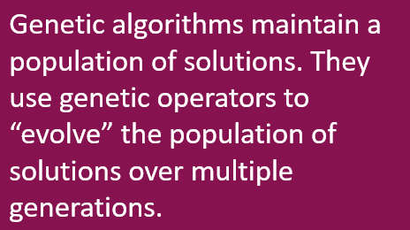
SAS’s black box optimization solver was formerly (prior to SAS Optimization 8.5) called the local search optimization LSO solver. It conducts a local search as well as global search algorithms. These are executed in parallel in CAS. Genetic algorithms provide the framework for black box optimization. The global and local search elements operate within that framework.

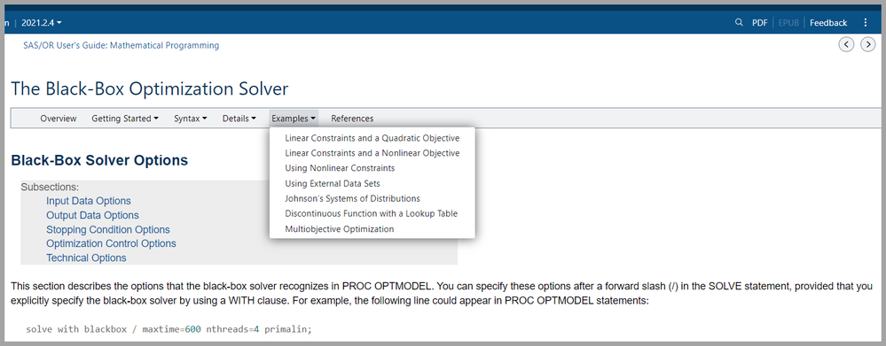
For example code to run the black box solver, follow the examples given in the documentation.

Select any image to see a larger version.
Mobile users: To view the images, select the "Full" version at the bottom of the page.

solveBlackbox CAS Action

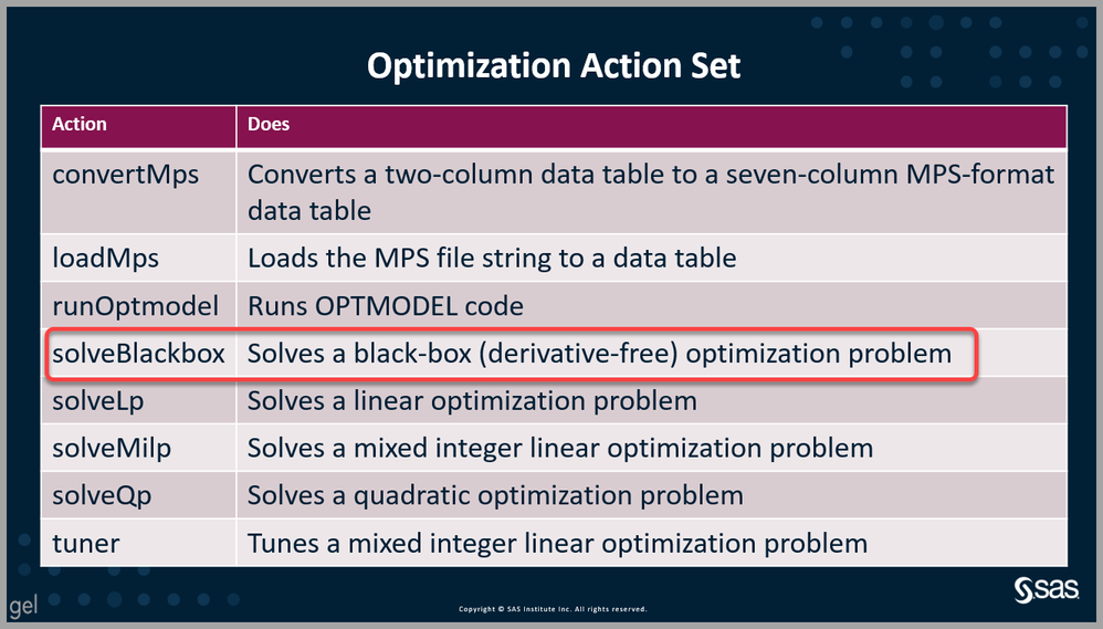
Using the solveBlackbox CAS action gives you more flexibility and also enables parallel function evaluations to call CASL code that runs in parallel. The solveBlackbox action is part of SAS’s Optimization Action Set.

Using CASL code you can employ action parameters to declare decision variables and linear constraints. You can also define nonlinear functions or constraints in EVAL subparameter. The solveBlackbox action enables parallel function evaluations to call code that runs in parallel. In the example below we illustrate using the eval subparameter of the func parameter as well as the nparallel parameter. Be aware that the eval=code block can call CAS actions to evaluate a nonlinear function; you cannot do this with PROC OPTMODEL. There is also an nSubsessionWorkers subparameter to the func parameter that specifies how many work nodes to allocate to each subsession that is evaluating an objective function.

Simple Example Using solveBlackbox For a very simple illustration for using the CAS action solveBlackbox, let’s use a common global optimization test function the six-hump camel back function. Within the bounded region are six local minima, two of them are global minima. This is an example of a mixed integer nonlinear program, with mix of binary and continuous decision variables, a nonlinear objective, and a mix of nonlinear and linear constraints.

The objective is to minimize:

Subject to:

See the code below:

Let’s review the log. We see that the data set CASUSER.CONSTRAINTS has 3 observations and 5 variables.

We see that the optimization action set was added, which includes solveBlackbox. Notice that unlike in Python, in CASL we don’t have to have a separate sess.loadactionset('optimization') statement to load the action set. Simply with the statement optimization.solveblackbox, the optimization action set is loaded, as shown in the log below. We can also see that the solveBlackbox action is using the Evolutionary Algorithms Guiding Local Search (EAGLS) optimizer algorithm and that it is executing 3 evaluations in parallel, each using one worker node. We can also see the interations one through ten.

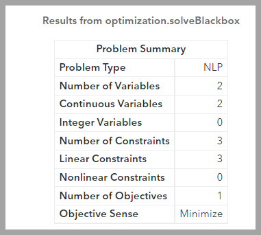
Looking at our results, we can see the problem summary, option summary, and solution summary. We see the problem type is nonlinear with 2 continuous constraints and 3 linear constraints. We have just one objective, to find the global minimum.

Next we see our max iterations is 10 and our number of local solvers is 4.

Finally we see our solution provides an objective of -1.02955 after 10 iterations and 172 evaluations. Not too bad!

Again, we see our objective is -1.02955.

In this case we know the global minima, which are -1.0316 at x = (0.0898, -0.7126) and (-0.0898, 0.7126). I hope I’ve piqued your interest in learning more about the optimization behind autotuning, and maybe even trying it out yourself! You can also use solveBlackbox to build a custom architecture or modify and improve a pre-built architecture and help you find the best model for your needs. See the resources below for more detailed information and examples.

For More Information

Extra Are you still wondering about the secret sauce in my Aunt Lonnie’s famous Irish Shepherd’s pie? That’s right, it’s Guinness! Didja na see that comin?

Find more articles from SAS Global Enablement and Learning here.

A Secret Sauce Behind SAS's Advanced AutoTuning: Black Box Optimization

Free course: Data Literacy Essentials

Get Started