Solved: Re: help with trimming independent variables in a confusing experiment... - Page 2

1zmm · Posted 08-28-2013 10:33 AM

After all of this discussion, I did not realize that exercise was a continuous variable. Your first message describing your question (August 14, 2013 at 4:41 pm) describes your 50 subjects as performing "20 different TYPES of exercise (vertical jump, . . .)", implying that exercise is a categorical/nominal variable with 20 different values. Now, it appears that exercise is a continuous value that measures the performance (in some units) on these different types of exercise. This distinction between a nominal and a continuous value is important because it would make a difference in the model. Obviously, continuous variables should NOT be placed in a CLASS statement but should be placed as a covariate/independent variable in the MODEL statement. Since you have already excluded EXERCISE from the CLASS statemnte (yesterday afternoon's message), that appears to be the appropriate approach to take. The error message/note that you received about an "infinite likelihood. . . because of a nonpositive definite estimated R matrix" is, according to the PROC MIXED documentation, "usually no cause for concern if the iterations continue". It may indicate that "observations from the same subject are producing identical rows" in the R matrix; that is, the same subject has duplicate covariates (VAR and TASK) in the PROC MIXED REPEATED statement. Check if and why this might be so. You might also use the R and the RCORR options of the REPEATED statement to print/display the first two blocks of the repeated-measures variance-covariance matrix and its corresponding correlation matrix (see the PROC MIXED REPEATED statement documentation: for example, R=1,2 and RCORR=1,2). To reduce memory requirements for PROC MIXED, you can also use the two other tips I suggested for reducing the time the procedure takes: Change the multivariate variance-covariance TYPE in the REPEATED statement from TYPE=UN@UN to TYPE=UN@CS, or make the categorical version of EXERCISE into a BY-variable and analyze the effect on the DVs through different TASKs of each kind of EXERCISE separately.

Ming · Posted 08-28-2013 04:24 PM

Hi,

I tried the model with r=1,2 and rcorr=1,2 and type=un@un or type=un@cs, all resulted in the same message, "an infinite likelihood is assumed in iteration 0 .... estimated R matrix for subject S02". so I printed the data to see if VAR and TASK have duplicated entries... here is the output for S02:

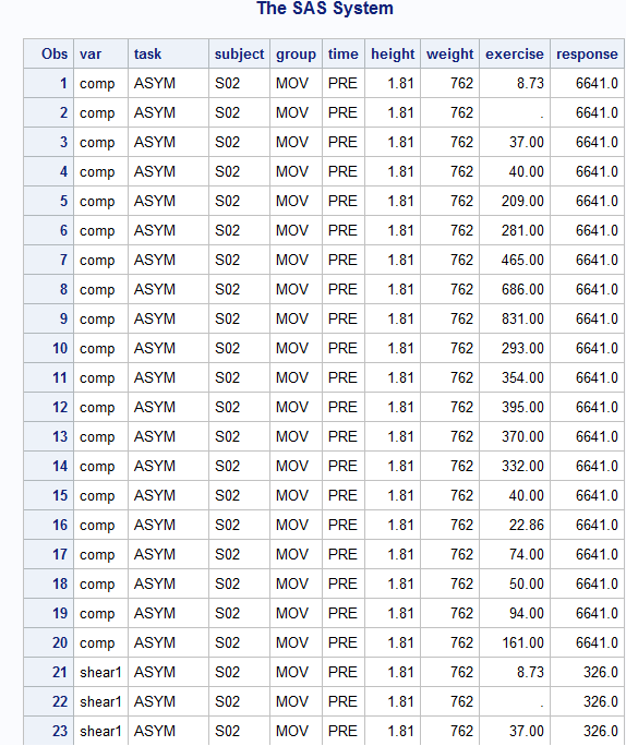
looks like VAR and TASK, in this case "comp" and "ASYM" are the duplicated 20 times for the exercise values. Is this why I'm getting the error message?

how can I circumvent around this? what about making the task*DV into one variable (called "trial") of 24 levels (task1_comp, task1_shear1, task1_shear2, task2_comp...), and the model statement will be:

model response = trial*exercise /s;

repeat trial / type=un;

will that work?

thanks.

ming

1zmm · Posted 08-31-2013 01:47 PM

I really don't understand your data. Within a particular subject at the same degree of RESPONSE, every variable except EXERCISE has the same value (for example, in subject S02). Because EXERCISE can vary by almost 100-fold (for example, from 8.73 to 831), although the value of the RESPONSE does not change (for example, COMP=6,641), EXERCISE should have no predictive power as an independent variable on this RESPONSE (and other responses as well). Perhaps you should model the RESPONSEs (COMP, SHEAR1, and SHEAR2) on the other independent variables that do NOT change--TASK, GROUP, TIME, HEIGHT, and WEIGHT. I do not see how the values of EXERCISE affect RESPONSE. I also don't understand what these values of EXERCISE represent since they appear to change while the values of the variables that do NOT change remain the same.

Ming · Posted 09-02-2013 02:54 PM

Hi,

Yeah, this experiment was really confusing... let me try to explain it a little better....

the main experiment is to have these subjects perform 8 tasks (SYMM, ASSYM, CPULL, PUSH,.....) and for each of the task, I took 3 measurements of their spine (compression, shear1 and shear2).

if this was all to the experiment, then I believe the analysis would be pretty straight forward MANOVA.

model comp shear1 shear2 = task;

However, there is another part to this experiment. The 50 subjects on a separate day did 20 different exercise tests (push up, sit up, vertical jump, hand grip strength....) and measurement for each exercise were recorded. So the question I have is... Can any of these exercises explain the variances of the 3 DVs (comp, shear1, shear2) in the first experiment?

hope this makes more sense now. I really appreciate your time/effort in helping me!

thanks.

ming

1zmm · Posted 09-02-2013 05:01 PM

Since the values for each of exercises and for each of the tasks are connected to the three dependent variables only through their occurring in the same study subject, the tasks are not really nested within the exercises or vice-versa. If you return to the original "short-but-wide" (few observations but many variables) data set with each of the values of the 20 exercises as a separate variable, you could include these exercises as independent variables in your model:

* Simple MANOVA model for each task alone;

proc glm;

class task;

model comp shear1 shear2=task / solution;

manova h=_all_ / printh printe summary;

run;

quit;

* Add in the 20 exercise variables;

proc glm;

class task;

model comp shear1 shear2=task exerc1-exerc20 / solution;

manova h=_all_ / printh printe summary;

run;

quit;

You can compare the r-squared statistic for each task alone on each of the three dependent variables or the statistic, 1 - Wilks' lambda, for the r-squared statistic for each task alone on all three of the dependent variables. Then see how much these r-squared statistics change when the 20 exercise variables are added to the model.

One problem with this approach is that you have very many independent variables (an intercetp term, seven indicator variables for the 8-category task variable, and 20 exercise variables) for relatively few study subjects (N=50); the regression coefficients for these independent variables may be very imprecise. PROC GLM will also delete observations when any of the dependent or independent variables are missing so that these analyses may be based on even fewer observations.

This approach also does not account for the fact that the observations for the tasks are correlated observations within each study subject; you'd have to use PROC MIXED again with the doubly multivariate approach to account for these within-subject correlations (see previous discussions).

A final problem with this approach is that it does not account for possible collinearity among the twenty exercise values. You could check this out by using the collinearity diagnostics available in PROC REG. Select only one observation from each study subject, and include all the exercises as independent variables in a model with any one of the three dependent variables as the dependent variable:

proc reg;

model comp=exerc1-exerc20 / collin;

run;

quit;

If any of the condition indexes in the collinearity diagnostics are 30 or more, then variables with "large" variance proportions are probably close to collinear. Then,

only one of these collinear values of exercise need to be in the model. PROC VARCLUS also "clusters" correlated variables, of which you can select one to represent all variables in a given cluster.

Message was edited by: Matthew Zack

Ming · Posted 09-02-2013 11:24 PM

Thanks for the explanations, makes much more sense now.

However I still don't know how to get around the PROC MIXED doubly multivariate error message an infinite likelihood is assumed in iteration 0 .... estimated R matrix for subject S02". Because it still sees subject s02 having multiple entries (ie exercise) for each task and response. How can I restructure the data so I can get around this error message?

thanks.

ming

SteveDenham · Posted 09-03-2013 08:40 AM

Try this:

proc mixed data=univariate;

class task var subject group exercise;

model response = var task group height weight ;

repeated var task / type=un@cs subject=subject(exercise);

run;

I realize that there are a gazillion (well, at least over 500) levels of exercise, but the only way to get rid of the infinite likelihood is to identify exercise within subject as the subject. See if this helps.

Steve Denham

Ming · Posted 09-03-2013 11:41 PM

still the same error...

NOTE: An infinite likelihood is assumed in iteration 0 because of a nonpositive definite estimated R matrix for subject(exercise)

S47 31.

here is the output:

The SAS System 23:37 Tuesday, September 3, 2013 1

The Mixed Procedure

Model Information

Data Set WORK.UNIVARIATE

Dependent Variable response

Covariance Structure Unstructured @ Compound

Symmetry

Subject Effect subject(exercise)

Estimation Method REML

Residual Variance Method None

Fixed Effects SE Method Model-Based

Degrees of Freedom Method Between-Within

Class Level Information

Class Levels Values

task 9 ASYM CBREACH CHOP CPULL FE HOH

PULL PUSH SYMM

var 3 comp shear1 shear2

subject 49 S02 S03 S04 S05 S06 S07 S08

S09 S10 S11 S12 S13 S14 S15

S16 S17 S18 S19 S20 S23 S25

S26 S28 S30 S31 S33 S34 S36

S39 S46 S47 S51 S55 S56 S57

S59 S60 S62 S63 S64 S65 S68

S69 S73 S74 S75 S78 S79 S80

group 3 CON FIT MOV

exercise 524 2.54 4.445 4.77 5.86 6.35 6.59

7.62 8.255 8.41 8.73 8.84 8.89

9.525 9.77 10 10.16 11.13 11.2

11.43 12 12.065 12.64 12.7

13.01 13.45 13.78 14.3 15

15.24 15.39 16 16.19 16.51

16.55 16.95 17 17.78 18 18.26

18.39 19.05 20 20.2 20.32

20.95 21.09 21.54 21.59 21.86

22.225 22.27 22.86 24 24.13

24.24 24.28 24.55 24.62 25

25.4 26.21 26.36 26.67 27

27.14 27.94 28 28.65 29 29.21

30 30.1 30.35 30.48 31 31.115

32 33 33.02 34 34.29 35 36 37

38 38.1 39 40 40.64 41 42 43

44 45 46 47 48 49 50 51 52 53

54 55 56 57 58 59 60 61 62 63

64 65 66 67 68 69 70 71 73 74

75 76 77 78 79 80 81 82 84 87

88 90 91 92 94 95 96 100 102

104 107 108 112 115 116 118

119 120 121 123 124 126 128

129 130 132 133 134 135 139

144 148 151 154 159 160 161

162 166 167 170 176 177 178

180 181 189 192 194 198 199

200 202 204 205 206 209 213

216 219 220 221 222 223 224

233 234 236 237 238 242 244

245 252 253 254 256 258 259

261 262 265 269 272 273 275

276 278 279 280 281 282 284

288 289 290 291 292 293 294

295 298 299 301 303 304 305

308 309 310 312 313 314 318

320 323 324 325 326 327 328

329 330 331 332 333 334 335

336 338 342 343 344 345 346

348 349 350 352 353 354 356

357 358 361 363 364 365 366

367 368 369 370 371 372 374

375 377 378 379 380 381 382

383 385 389 390 393 394 395

396 397 398 399 400 401 402

403 404 405 407 408 409 412

413 414 416 418 419 420 423

424 426 427 428 429 430 431

432 436 438 440 442 444 448

449 450 451 452 453 456 457

458 459 462 464 465 467 471

474 476 479 480 483 486 488

489 495 498 499 502 503 504

505 507 510 515 516 520 521

524 526 527 531 540 544 546

549 551 553 555 570 571 579

580 584 587 590 591 596 597

599 600 603 606 614 619 622

623 624 629 630 633 634 640

643 645 646 650 651 654 656

657 658 660 662 664 665 667

668 670 674 676 686 690 703

704 705 708 720 728 737 738

739 745 764 767 771 779 780

786 800 805 807 813 819 820

830 831 832 837 841 845 852

858 860 867 874 875 877 878

881 882 885 887 891 908 912

913 916 919 921 927 929 930

935 941 948 956 962 970 979

998 1008 1028 1032 1046 1047

1050 1055 1063 1072 1089 1091

1095 1096 1104 1108 1109 1120

1121 1138 1140 1141 1150 1161

1163 1171 1172 1175 1178 1189

1197 1211 1220 1227 1236 1274

1303 1410 1473 1555

Dimensions

Covariance Parameters 7

Columns in X 18

Columns in Z 0

Subjects 934

Max Obs Per Subject 81

Number of Observations

Number of Observations Read 29100

Number of Observations Used 25524

Number of Observations Not Used 3576

1zmm · Posted 09-04-2013 07:19 AM

Your experiment does not really have 934 subjects, only 50.

Back on August 22nd, I sent some code that might be modified (see below) and work without error messages about infinite likelihoods. Although PROC MIXED does not print an R-squared statistic as PROC GLM does, the IC option on the PROC MIXED statement will have SAS print various information criteria that allow you to compare the two approximately nested models (without and with the various values for the twenty exercise variables). I also include a PROC REG paragraph to check for collinearity among the exercise variables and a PROC VARCLUS paragraph to see if the exercise variables group into correlated variable clusters.

Matthew Zack

=========================================================================================================================

* The first two of these procedures assume that only one observation per study subject is selected;

* and that this observation contains the values for all 20 exercise variables.;

* If this is false, then select only one observation per study subject in prior code (see below).;

* Sort the original, WIDE data set;

* by study subject;

proc sort data=wide;

by subject;

run;

* Select only one of the study subjects into a new data set;

* for analysis of the collinearity statistics and variable clustering;

* of the exercise variables.;

data wide2;

set wide;

by subject;

if (first.subject eq 1)

then output wide2;

run;

* Check the exercise variables for collinearity.;

* Because these collinearity diagnostics are relevant only to the independent variables,;

* the value of the dependent variable is not relevant.;

proc reg data=wide2;

model comp=exerc1-exerc20 / collin;

title10 "Collinearity diagnostics for the 20 exercise variables";

run;

quit;

* Check if the exercise variables group into clusters of correlated variables;

proc varclus data=wide2;

var exerc1-exerc20;

title10 "Check if the exercise variables group into clusters of correlated variables";

run;

* For each dependent variable, use the original, WIDE data set to creata a separate dependent variable;

* with the same name, RESPONSE, but indexed by the variable, VAR.;

data long(drop=j comp shear1 shear2);

length var $ 12;

set wide;

array dv{3} comp shear1 shear2;

array varlist{3} $ 12 _temporary_ ("comp" "shear1" "shear2");

do j=1 to 3;

response=dv{j};

var=varlist{j};

output long;

end;

run;

* Sort data;

* by subject, task, and distinct dependent variable;

proc sort data=long;

by subject task var;

run;

* Model dependent variables as multivariate repeated measures;

* Determine the effects of the task on the response;

* May vary the REPEATED statement variance-covariance matrix from TYPE=UN@CS to TYPE=UN@UN;

proc mixed data=long ic;

class subject task var;

model response = var task var*task

/ solution ddfm=kenwardroger;

repeated var task / type=un@cs subject=subject rcorr;

run;

quit;

* Model dependent variables as multivariate repeated measures;

* Determine the effects of the task and the exercise values on the response;

* May vary the REPEATED statement variance-covariance matrix from TYPE=UN@CS to TYPE=UN@UN;

proc mixed data=long ic;

class subject task var;

model response = var task var*task exerc1-exerc20

/ solution ddfm=kenwardroger;

repeated var task / type=un@cs subject=subject rcorr;

run;

quit;

Ming · Posted 09-04-2013 11:29 PM

Hi,

it finally converged! I had to remove the interaction term (var*task) for this to happen. I think it is reasonable to remove it since var and task shouldn't be interacted since var are the DVs.

Looking at the output, none of the 20 exercises (except for exerc7) showed any significance contribution to the model, so does that mean I should run a model with all the exercises (and keep only exerc7) removed and compare the AIC numbers between the two to see which is a better model? To answer my initial question, can the 20 exercises predict the comp/shear loading on lower back? Based on all the non-significant exerc results, it is fair to say that only 1 exercise contribute significantly in explaining the variances in comp/shears loading.

Can I eliminate the 20 exercises based on the VIF (proc reg) number? basically only take those exercises that's VIF<10 and put them in the model.

thanks.

ming

This is the output:

The Mixed Procedure

Model Information

Data Set WORK.UNIVARIATE

Dependent Variable response

Covariance Structure Unstructured @ Compound

Symmetry

Subject Effect subject

Estimation Method REML

Residual Variance Method None

Fixed Effects SE Method Model-Based

Degrees of Freedom Method Between-Within

Class Level Information

Class Levels Values

task 9 ASYM CBREACH CHOP CPULL FE HOH

PULL PUSH SYMM

var 3 comp shear1 shear2

subject 32 S03 S04 S05 S07 S08 S09 S10

S14 S16 S18 S19 S20 S23 S25

S26 S28 S30 S31 S33 S34 S39

S46 S47 S56 S57 S59 S60 S62

S65 S68 S74 S78

Dimensions

Covariance Parameters 7

Columns in X 35

Columns in Z 0

Subjects 32

Max Obs Per Subject 27

Number of Observations

Number of Observations Read 1455

Number of Observations Used 855

Number of Observations Not Used 600

Iteration History

Iteration Evaluations -2 Res Log Like Criterion

0 1 14792.77345721

1 2 13189.65467530 0.51939632

2 1 13189.22649090 0.00957869

3 1 13189.21664571 0.00000590

4 1 13189.21656394 0.00000000

Convergence criteria met but final hessian is not positive

definite.

Covariance Parameter Estimates

Cov Parm Subject Estimate

var UN(1,1) subject 5579892

UN(2,1) subject -1947614

UN(2,2) subject 955329

UN(3,1) subject -2011194

UN(3,2) subject 968609

UN(3,3) subject 1015267

task Corr subject -0.00282

Fit Statistics

-2 Res Log Likelihood 13189.2

AIC (smaller is better) 13203.2

AICC (smaller is better) 13203.4

BIC (smaller is better) 13213.5

Null Model Likelihood Ratio Test

DF Chi-Square Pr > ChiSq

6 1603.56 <.0001

Type 3 Tests of Fixed Effects

Num Den

Effect DF DF F Value Pr > F

var 2 62 463.50 <.0001

task 8 245 178.98 <.0001

height 1 9 0.14 0.7128

weight 1 9 4.98 0.0526

exerc1 1 9 0.89 0.3693

exerc2 1 9 0.01 0.9320

exerc3 1 9 0.24 0.6364

exerc4 1 9 0.04 0.8453

exerc5 1 9 0.11 0.7478

exerc6 1 9 2.10 0.1809

exerc7 1 9 7.96 0.0200

exerc8 1 9 0.00 0.9512

exerc9 1 9 1.93 0.1986

exerc10 1 9 0.03 0.8625

exerc11 1 9 0.78 0.3998

exerc12 1 9 0.08 0.7818

exerc13 1 9 0.29 0.6045

exerc14 1 9 0.10 0.7617

exerc15 1 9 2.14 0.1778

exerc16 1 9 3.14 0.1099

exerc17 1 9 1.73 0.2206

exerc18 1 9 0.73 0.4142

exerc19 1 9 0.05 0.8306

exerc20 1 9 2.23 0.1695

1zmm · Posted 09-05-2013 08:33 AM

This output shows that the results for only 32 study subjects and only 855 out of 1,455 observations were used in the PROC MIXED analysis. This loss seems somewhat excessive. In previous abbreviated lists of data on this Internet site, a few variables had missing values. Do you think that this is why so many observations were excluded from the analysis? It may be worthwhile to check the pattern of missing dependent variables and independent variables to determine whether you can exclude some variables with large percentages of missing values from the analysis. For example, you can display the pattern of missing values by using the procedure, PROC MI, as follows:

proc mi nimpute=0;

var y var task height weight exerc1-exerc20;

run;

quit;

I followed the PROC MIXED documentation for the MODEL statement syntax including the VAR*TASK interaction as an independent variable (see the documentation for the REPEATED statement option, TYPE, for multivariate repeated measures. However, if the model that includes this VAR*TASK interaction does NOT converge, and if the model that excludes this interaction DOES converge, then the latter model may be the way to go. Another alternative model would be to use the MODEL statement that includes only the VAR*TASK interaction without including the main-effect terms, VAR or TASK, as independent variables (the "cell means" model):

model response=var*task height weight . . . .;

I prefer to use the condition number rather than the VIF statistic in PROC REG to identify groups of highly correlated independent variables. A condition number of 30 or more (10 or more in models without intercept terms) and independent variables with relatively large variance proportions will identify such group(s). Then, from subject matter knowledge or from the use of PROC VARCLUS to group highly correlated variables, you can select one or a few variables within each group to represent all the highly correlated variables in the group for use as independent variables in subsequent modelling.

Since only one of the 20 exercises (exerc7) remained statistically significantly associated with the response after adjusting for VAR and TASK, this specific exercise may or may not be substantively associated with the response (perhaps a multiple comparison problem); perhaps subject-matter knowledge about what this exercise represents will help you to decide whether to keep it in the model or not. However, to decide whether or not to include it in your assessment of the value of these exercises in predicting the response by comparing the information criteria of different models, I would compare the model having only VAR, TASK, WEIGHT, and HEIGHT as independent variables with the model having VAR, TASK, WEIGHT, HEIGHT, and all 20 of the exercise variables (not just EXERC7) because you didn't have any a priori reason to select only EXERC7.

Ming · Posted 08-28-2013 05:22 PM

now exercise is a continuous variable, does this change the analysis for PROC GLM?

data long; set wide;

array e(20) exerc1-exerc20;

do i = 1 to 20;

exercise = i;

exerc = e(i);

output;

end;

drop i time exerc1-exerc20;

proc glm data=long;

title 'task/exercise manova';

class task exercise;

model std_comp std_shr1 std_shr2 = task(exercise) /solution;

manova h=_all_ /printe printh summary;

looks like the values for "exerc" are not being used in the analysis, task(exercise) are being treated as nominal variable. I tried adding exerc as a covariate by:

model std_comp std_shr1 std_shr2 = task(exercise)|exerc /solution;

does this look right?

thanks.

ming