- Home
- /
- SAS Communities Library
- /
- Wavelet Analysis using SAS/IML: Thresholding the Detail Coefficients t...
- RSS Feed
- Mark as New
- Mark as Read
- Bookmark
- Subscribe
- Printer Friendly Page
- Report Inappropriate Content
Wavelet Analysis using SAS/IML: Thresholding the Detail Coefficients to Remove High-Frequency Noise
- Article History
- RSS Feed
- Mark as New
- Mark as Read
- Bookmark
- Subscribe
- Printer Friendly Page
- Report Inappropriate Content
The purpose of this blog is to learn how wavelets can be used to remove unwanted high-frequency noise from digital signals. Wavelets can be used to decompose a signal into different frequency components (with different resolutions at each frequency level), and once we have the decomposition, we can manipulate the high-frequency component of the signal to reduce or eliminate the noise. This can be useful to clean up sensor data with unexpected high frequency noise. An example of this is a vibration sensor on a spinning turbine that generates an electromagnetic signal, but the signal experiences electromagnetic interference before it is read into a computer. The output digital signal includes both the actual vibration data, and some unwanted electromagnetic noise riding on top of the signal.
The basic process for this is to calculate the wavelet decomposition coefficients, and then apply some kind of threshold to the wavelet detail coefficients (the coefficients for the high-frequency components of the signal) to shrink their magnitude (soft thresholding) or reduce them to zero (hard thresholding). We will describe this process in detail in this blog and we will see examples of applying this to simulated and real data using the wavelet tools in the SAS Interactive Matrix Language.
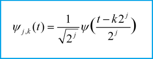
In a previous blog on wavelet analysis (link provided below), we introduced the discrete wavelet transform and showed the following equation for a family of wavelets at different shift and scale parameters (scaling by powers of two):
The scale parameter j determines the frequency of the wavelet, while the shift parameter k determines the temporal support for the wavelet. As we increase k, we are moving the wavelet forward in time (to the right on a plot) across the input signal. As we increase j, the frequency of the wavelet increases and thus we capture higher frequency variation in the signal using wavelets with larger values of j. The wavelet transform yields a collection of coefficients representing the information in the signal corresponding at different shifts and scales, with one coefficient for each wavelet (each pair of values of k and j define a wavelet and thus correspond to one coefficient). The coefficients are thus spread out in time and frequency, with different values of k corresponding to the signal components at different times, and different values of j corresponding to the signal frequency contents. The coefficients for high values of j are called the “detail coefficients” and represent the high-frequency components in the signal. We will threshold these detail coefficients to eliminate some of the high-frequency components and thus remove unwanted high-frequency noise.
Let’s explore an example of removing low-amplitude, high-frequency noise from a simulated sinusoidal signal. This is a very simple toy example (most real-world signals are not perfect sinusoids with perfect sinusoidal noise) but it provides good intuition for how the denoising operation works. We start by simulating the input signal and the additive noise using SAS/IML:
proc iml;
/*We start by simulating a digital signal with a small amplitude high-frequency noise injected*/
    f_s = 500; /*sampling frequency*/
    f_s2 = f_s/2; /*Nyquist frequency*/

    t_s = 1/f_s; /*sampling period (time between samples)*/
    N_samp = 1000; /*number of samples*/

    t = do(0, (N_samp-1)*t_s, t_s);
    fS = 2;
    fN = 225;
    pi = constant("pi");

    x_Signal = sin(2*pi*fS*t); /*Signal component*/
    x_Noise = 0.05*sin(2*pi*fN*t); /*Noise component*/
    x_NoisySignal = x_Signal+x_Noise;

    create work.input_signal var {"t","x_NoisySignal","x_Signal","x_Noise"};
    append;
    close work.input_signal;

/*plot our signal in the time domain*/
    submit;
    title "Input Digital Signal with and without Noise";
    proc sgplot data=work.input_signal;
        series x=t y=x_NoisySignal;
        series x=t y=x_Signal;
        xaxis grid label="Time (s)";
        yaxis grid label="Amplitude";
        legend;
        run;
    endsubmit;
run;
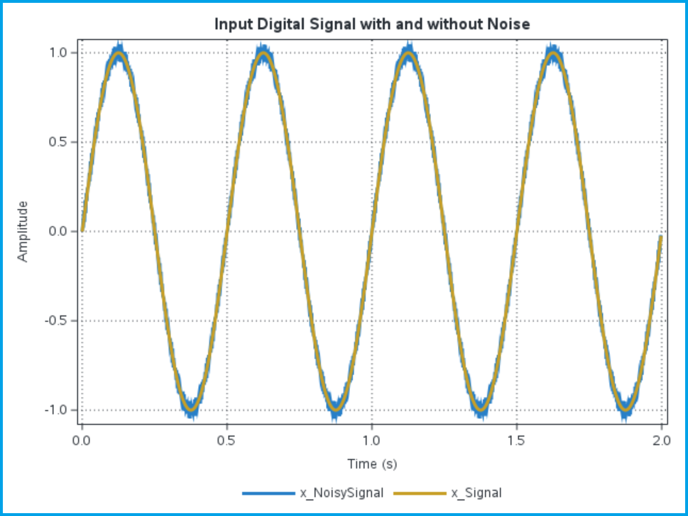
Note that in this example the input signal has a frequency of 2 Hz, while the additive noise has a frequency of 225 Hz. The noise is also much smaller than the signal in this example, with an amplitude of 5% the signal amplitude. This yields the following plot, showing the noise-free input signal overlaid on top of the actual noisy signal we will analyze:
Our goal is to reconstruct the original noise-free signal (x_Signal in the plot) from the ‘measured’ input signal with noise (x_NoisySignal in the plot). In this example we are imagining we don’t have access to the noise-free signal, and the only thing we have is the measured data, x_NoisySignal. We start by performing the discrete wavelet transform to calculate the wavelet decomposition, and then we plot the detail coefficients so we can explore them before we apply any kind of thresholding (note that this code is still in the same call to PROC IML as the previous block of code. Listed macro and function calls are described below):
    /*now let's calculate the wavelet decomposition so we can threshold the wavelet detail coefficients*/
    %wavinit;
    /*let's use a predefined Daubechies 3-tap wavelet*/
    optn = &daubechies3;

    /*now perform the discrete wavelet transform to find the decomposition*/
    call wavft(decomp, x_NoisySignal, optn);

    call wavprint(decomp, &detailCoeffs, 1, 4);

    call coefficientPlot(decomp);

    call coefficientPlot(decomp, &SureShrink);

run;
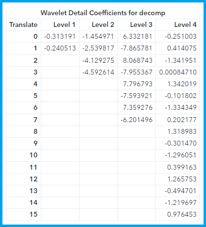
The %wavinit macro is used to setup the wavelet functions we will use to streamline the submission of the wavelet analysis code. This code allows us to define our wavelet family and type using the macro variable &daubechies3 (as opposed the syntax we would use without the %wavinit macro which would require looking up all of the numeric options in the SAS documentation and specifying each option by number). The function call to wavft calculates the wavelet decomposition, but we will use other wavelet analysis functions to extract the relevant information from this decomposition. We start by printing the detail coefficients at level 1-4 using the wavprint call function. This yields the following table of coefficients:
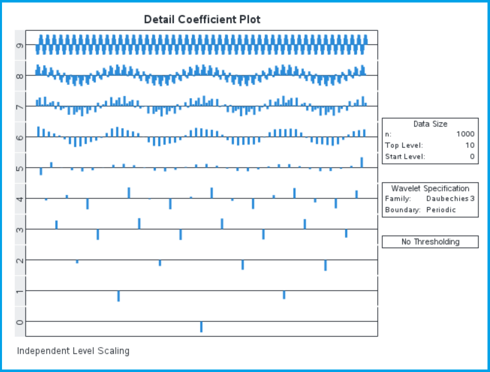
The different value of the Translate column correspond to different shift values, but they fill the time domain for each level. Although the values of Translate represent the shift k, they don’t correspond to the actual shift value in time. In this way the two detail coefficients at level 1 cover the same time domain as the four detail coefficients at level 2, we just have greater time resolution at the higher levels. This table only shows the first four levels of detail coefficients, but with our default settings we calculate 10 levels of detail coefficients (levels 0 to 9). We want to apply a threshold to the higher-level detail coefficients, but there are too many of them to explore in a table, so we plot them:
This plot clearly illustrates how the detail coefficients are distributed in time (with greater time resolution for the more numerous high frequency detail coefficients). We haven’t applied thresholding yet, so we can see the high-frequency variation in the higher levels of detail coefficients. This plot also highlights the time-frequency resolution discussed in the previous blog on wavelet scalograms, with greater time resolution at higher frequencies (although it doesn’t highlight the corollary to this, which is that we have lower frequency resolution at higher frequencies as well).
We can apply either soft thresholding to these coefficients to shrink them in magnitude, or hard thresholding to set some of the coefficients to exactly zero. We use the &SureShrink option in SAS/IML to apply soft thresholding to these detail coefficients, although we could also try out the &RiskShrink option to apply hard thresholding. The software allows us to use more customized thresholding options, but the developers include macro variables in the wavelet toolkit to make it easier to apply popular thresholding methods. After applying the soft thresholding, we can plot the transformed detail coefficients:
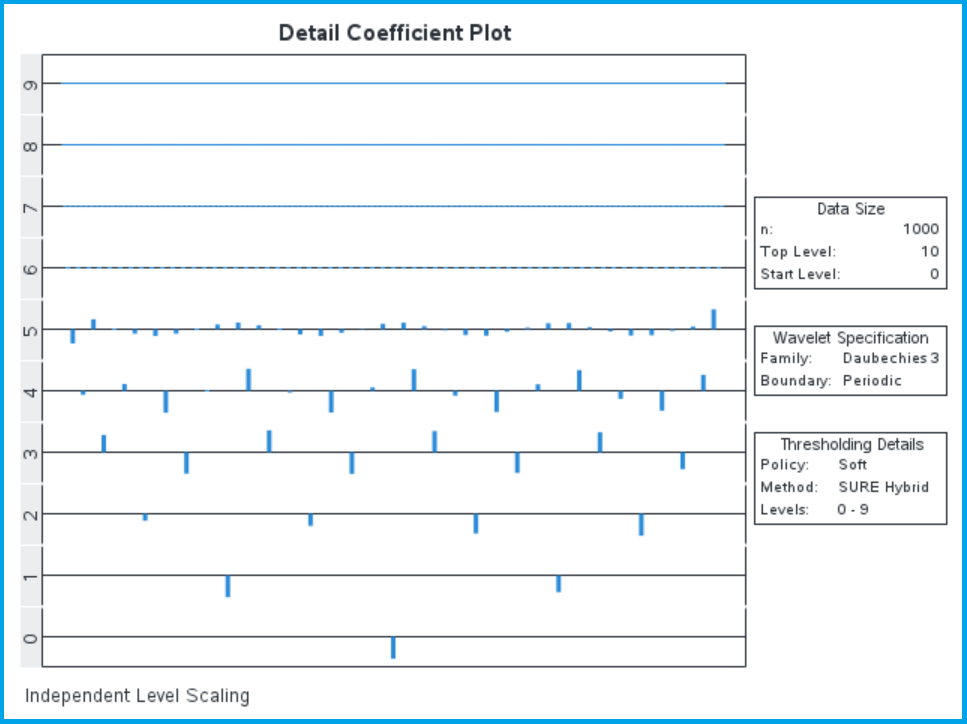
It looks like the detail coefficients at levels 6, 7, 8, and 9 have been set to zero, although we used a soft threshold, so they have actually just been shrunk to the point where they are not visible on the plot. We can see that most of the high-frequency variation we saw in the detail coefficients at the higher levels is absent from the plot, so we can expect that this thresholding has removed most of the high-frequency noise. To investigate this, we must perform the inverse wavelet transform on the decomposition with the modified detail coefficients:
    call wavift(x_denoised, decomp, &SureShrink);

    x_diff = x_signal - x_denoised;

    /*create an output dataset to plot the results*/
    create work.denoised_signal var {"t","x_NoisySignal","x_Noise","x_Signal", "x_denoised", "x_diff"};
    append;
    close work.denoised_signal;

    submit;
    /*first we plot the denoised signal*/
    title "Denoised Signal";
    proc sgplot data=work.denoised_signal;
        series x=t y=x_denoised;
        xaxis grid label="Time (s)";
        yaxis grid label="Amplitude";
    run;

    /*now we plot the difference between the original "noise-free" signal and the denoised signal*/
    title "Difference between original noise-free signal and denoised signal";
    proc sgplot data=work.denoised_signal;
        series x=t y=x_diff;
        xaxis grid label="Time (s)";
        yaxis min=-1 max=1 grid label="Amplitude";
    run;
    endsubmit;
quit;
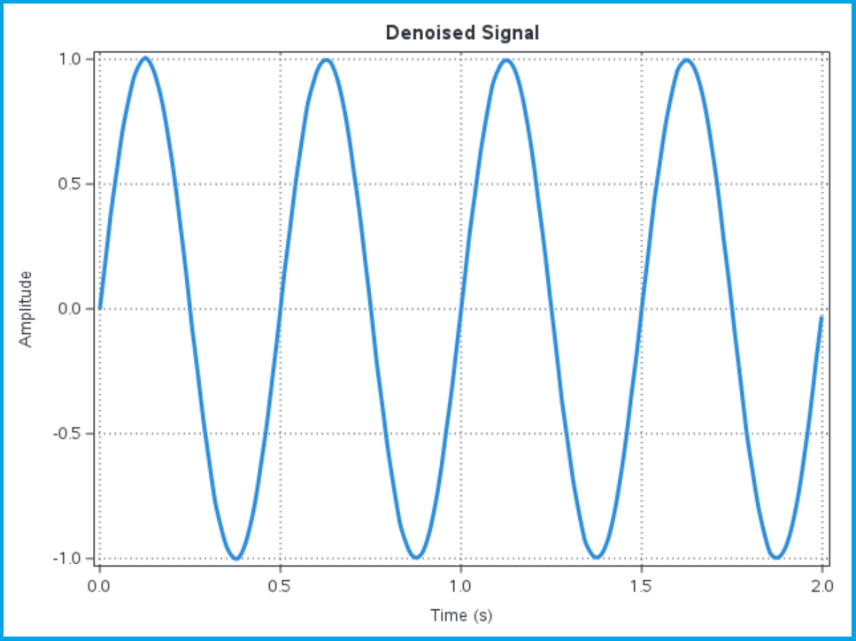
The wavift call performs the inverse wavelet transform to create the output signal x_denoised from the wavelet decomposition decomp, using the &SureShrink method to threshold the wavelet detail coefficients. After we create the denoised signal, we calculate a difference between the original noise free signal and the denoised signal to evaluate the effectiveness of the wavelet denoising approach. We plot the denoised signal along with the difference between the denoised signal and the original noise-free signal to compare:
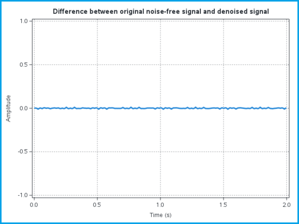
Visually the denoised signal looks like our original signal; it no longer has the high-frequency variation we saw on the noisy signal. Of course, the plot can be misleading, so we can also plot the difference between the denoised signal and the original noise-free signal:
We can see that the denoised signal is not exactly equal to the original noise-free signal, and the deviations seem to be somewhat periodic in time (which makes sense given the periodic nature of the wavelet analyses).
This toy example is just a simple sinusoid, but wavelet denoising is especially useful when the data contains sharp transitions or jumps, something that is very common in real world sensor and signal data. Traditional Fourier transform methods can also be used to remove high-frequency noise (discussed in a previous blog post, link below), but the basis used for the Fourier transform (sines and cosines) does a bad job representing sharp transitions or level shifts. Any attempt to use a Fourier transform to remove high-frequency noise will also invariably smooth out and modify these sharp transitions. This is a problem because these sharp transitions are not high-frequency noise components, and they often represent times when important events occurred in the data, so we want to preserve the temporal location of these transitions. Wavelet analysis is a powerful tool in these scenarios because the wavelet transform can remove the high-frequency noise without smoothing or eliminating regions where the signal experiences a level shift or a sharp transition.
References:
Available on demand!
Missed SAS Innovate Las Vegas? Watch all the action for free! View the keynotes, general sessions and 22 breakouts on demand.
Free course: Data Literacy Essentials
Data Literacy is for all, even absolute beginners. Jump on board with this free e-learning and boost your career prospects.
Get Started
- Find more articles tagged with:
- GEL
- SAS IML
- Signal Processing
- Wavelets
