testing for a negative correlation between 2 dependent variables in a repeated measures analysis

[palolix]

Steve, I was doing a mistake, because I was using the residual option with the beta and the binomial dist, and for distributions where the mean and variance are functionally related you should  not use the residual option.  So now I get negative values with the binomial dist for the prop of healthy vs prop diseased eggs and Gener. Chi-Square / DF=0.08

1	1.0000		-337E-24		9.25E-26		-148E-31		5.01E-33
2		1.0000		-84E-22		2.3E-24		-369E-30		1.25E-31
3	-337E-24		1.0000		-346E-24		5.55E-26		-187E-31
4		-84E-22		1.0000		-863E-23		1.38E-24		-467E-30
5	9.25E-26		-346E-24		1.0000		-271E-24		9.18E-26
6		2.3E-24		-863E-23		1.0000		-676E-23		2.29E-24
7	-148E-31		5.55E-26		-271E-24		1.0000		-262E-24
8		-369E-30		1.38E-24		-676E-23		1.0000		-653E-23
9	5.01E-33		-187E-31		9.18E-26		-262E-24		1.0000
10		1.25E-31		-467E-30		2.29E-24		-653E-23		1.0000
11											1.0000		-301E-24		6.43E-26		-162E-31		4.12E-33
12												1.0000		-749E-23		1.6E-24		-404E-30		1.03E-31
13											-301E-24		1.0000		-342E-24		8.62E-26		-219E-31
14												-749E-23		1.0000		-852E-23		2.15E-24		-546E-30
15											6.43E-26		-342E-24		1.0000		-329E-24		8.37E-26
16												1.6E-24		-852E-23		1.0000		-82E-22		2.08E-24
17											-162E-31		8.62E-26		-329E-24		1.0000		-376E-24
18												-404E-30		2.15E-24		-82E-22		1.0000		-936E-23
19											4.12E-33		-219E-31		8.37E-26		-376E-24		1.0000
20												1.03E-31		-546E-30		2.08E-24		-936E-23		1.0000

Although there is no significant interaction including eggtype in the table for fixed effects.

Thanks Steve!!

[SteveDenham]

But you aren't getting negative values.  The off diagonal values are all zeroes to the extent of machine accuracy, and may show as almost anything.

So to look at counts and proportions in the same analysis, look at Example 44.5 Joint Modeling of Binary and Count Data (may have a different example number, depending on version of SAS/STAT.  This is for 13.2).  In particular, take a look at the very last set of code for a marginally correlated error model.

Steve Denham

[palolix]

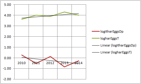
I see. Anyhow, when I plot the data, it doesn´t look like there is really a neg corr with log and logit transformed counts and proportions, eventhough the oscillations seems to be opposite

Thank you so much for all your great help Steve!

Caroline

[palolix]

Hi again Steve,

I found a correlation that seems to be positive, but how to get the p-values under each corr coefficient in order to determine if they are significant? Is there a statement that I can include in my code?

Proc glimmix data=one;

class nem blk year eggtype;

model Eggs= eggtype|nem|year/dist=lognormal ddfm=kr;

random intercept/subject=blk;

random year/residual subject=blk*nem type=ar(1) group=eggtype vcorr;

run;

Thank you dear Steve!

Caroline

[SteveDenham]

Not in GLIMMIX.  I think the best you can do will be to export to a dataset, apply Fisher's transformation (hyperbolic arctangent) and get a z-score, using the residual degrees of freedom, rather than the n - 3 for the standard analysis.

Steve Denham

[palolix]

You have a solution for everything Steve!

Thank you so much for all your wonderful help!!

Caroline

[SteveDenham]

Not really--I've just been doing a lot of this stuff for a long time.

Steve Denham

[palolix]

I tried healthy eggs with disease eggs. Significant interactions including eggtype, but still no negative values. I also compared proportion of healthy eggs with proportion of disease eggs, but no negative values.

I would appreciate if you could have a look, maybe I am doing something wrong. (harEggsT means he number of total eggs. I also divided 4 because I need the numbers in 100g soil and he raw data is in 400g)

data one;

input nem$ blk$    year eggtype$ harEggs harEggsT;

harEggs=harEggs/4;

harEggs=harEggs+1;

harEggsT=harEggsT/4;

harEggsT=harEggsT+1;

harPerEggs=100*harEggs/harEggsT;

cards;

Chav    A    2010    healthy    1400    8700

Chav    A    2010    diseased    7300    8700

Chav    A    2011    healthy    27375    35250

Chav    A    2011    diseased    7875    35250

Chav    A    2012    healthy    9700    27900

Chav    A    2012    diseased    18200    27900

Chav    A    2013    healthy    60625    68875

Chav    A    2013    diseased    8250    68875

Chav    A    2014    healthy    19350    34425

Chav    A    2014    diseased    15075    34425

Chav    B    2010    healthy    3000    10800

Chav    B    2010    diseased    7800    10800

Chav    B    2011    healthy    17100    21700

Chav    B    2011    diseased    4600    21700

Chav    B    2012    healthy    11625    28275

Chav    B    2012    diseased    16650    28275

Chav    B    2013    healthy    71750    81500

Chav    B    2013    diseased    9750    81500

Chav    B    2014    healthy    25500    46800

Chav    B    2014    diseased    21300    46800

Chav    C    2010    healthy    27200    36000

Chav    C    2010    diseased    8800    36000

Chav    C    2011    healthy    44250    66500

Chav    C    2011    diseased    22250    66500

Chav    C    2012    healthy    13500    26500

Chav    C    2012    diseased    13000    26500

Chav    C    2013    healthy    82800    97650

Chav    C    2013    diseased    14850    97650

Chav    C    2014    healthy    29400    38300

Chav    C    2014    diseased    8900    38300

Chav    D    2010    healthy    5600    22400

Chav    D    2010    diseased    16800    22400

Chav    D    2011    healthy    43500    53100

Chav    D    2011    diseased    9600    53100

Chav    D    2012    healthy    17800    43900

Chav    D    2012    diseased    26100    43900

Chav    D    2013    healthy    62200    70600

Chav    D    2013    diseased    8400    70600

Chav    D    2014    healthy    35125    47875

Chav    D    2014    diseased    12750    47875

Delm    A    2010    healthy    800    12600

Delm    A    2010    diseased    11800    12600

Delm    A    2011    healthy    2850    24750

Delm    A    2011    diseased    21900    24750

Delm    A    2012    healthy    9150    34200

Delm    A    2012    diseased    25050    34200

Delm    A    2013    healthy    21500    30000

Delm    A    2013    diseased    8500    30000

Delm    A    2014    healthy    8750    16850

Delm    A    2014    diseased    8100    16850

Delm    B    2010    healthy    7000    46800

Delm    B    2010    diseased    39800    46800

Delm    B    2011    healthy    28000    62000

Delm    B    2011    diseased    34000    62000

Delm    B    2012    healthy    12400    41200

Delm    B    2012    diseased    28800    41200

Delm    B    2013    healthy    28350    37275

Delm    B    2013    diseased    8925    37275

Delm    B    2014    healthy    50300    72100

Delm    B    2014    diseased    21800    72100

Delm    C    2010    healthy    17250    55050

Delm    C    2010    diseased    37800    55050

Delm    C    2011    healthy    44700    88650

Delm    C    2011    diseased    43950    88650

Delm    C    2012    healthy    9400    51700

Delm    C    2012    diseased    42300    51700

Delm    C    2013    healthy    54375    89750

Delm    C    2013    diseased    35375    89750

Delm    C    2014    healthy    28200    56700

Delm    C    2014    diseased    28500    56700

Delm    D    2010    healthy    .    .

Delm    D    2010    diseased    .    .

Delm    D    2011    healthy    .    .

Delm    D    2011    diseased    .    .

Delm    D    2012    healthy    .    .

Delm    D    2012    diseased    .    .

Delm    D    2013    healthy    .    .

Delm    D    2013    diseased    .    .

Delm    D    2014    healthy    .    .

Delm    D    2014    diseased    .    .

Proc glimmix data=one;

harPerEggsp=harPerEggs/100;

class nem blk year eggtype;

model harPerEggsp= eggtype|nem|year/dist=beta ddfm=kr;

random intercept/subject=blk;

random year/residual subject=blk*nem type=ar(1) group=eggtype vcorr;

run;

Thank you very much Steve!!