Glimmix model for trap catch

[Hornet1937]

Hi all,

I have a working glimmix model for repeated insect trapcatch by habitat treatment. Code was written with the help of a university statistician. They strongly suggested that I use glimmix but they do not use the dist=KEYWORD model option. They pre-transform for normality instead. I would like to utilize this feature of the PROC but all attempts to write the code comes up with non-convergence, starting values of MISQUE, or non-significance problems.  Further down the road, I would like to add additional variables (specifically continuous ones), but I figured I ought fix this issue first. I have strong Excel skills but I am poor at SAS language and as a results I do things differently than I should. Further, I did not set up the experimental design and it was done very messy. I will try to explain as clearly as possible.

The response is number of insects caught, Total_Earwigs. The experimental design has four random 'blocks' but there are two different varieties 'Cultivars' of the sampling unit (a tree). Cultivar 1 is in block 1 and 3, Cultivar 2 was planted in block 2 and 4. The researchers who set up the experiment assumed that the cultivar has no affect on any responses and I nested it into block. Each block has 6 plots of different treatments 'trt_name' (6 levelsx4reps). Each plot has 15 trees and a randomly chosen tree had a two traps attached to it. When I collected the data I had assumed that tree within plot has no affect on responses and am choosing to ignore it for now. 'Forder' is a dummy variable corresponding to treatment that I threw in there to sort by and have the treatments 'trt_name' be ordered a specific way in graph outputs (not alphabetical). 'Year' has four levels. I trapped weekly but recorded time with unique units degree days (time spent within a species-specific temperature range). 'DD_Mean' refers to degree days but given that it was a continuous variable, I transformed the data into 6 discreet categories and averaged among those. The model is below and I have follow-up questions below.

proc import out=work.earwig dbms=tab replace

  datafile="&folder\&dataname";

  getnames=yes;

  datarow=2;

run;

proc sort data=earwig;

    by block cultivar   Forder Trt_Name Year DD_Mean;

proc means data=earwig (where=(Orchard=1 and DD_Mean<1750)) noprint;

    by block cultivar   Forder Trt_Name Year DD_Mean;

    var Total_Earwigs;

    output out= earwig_2 mean=Total_Earwigs;

    run;

data earwig_2;

    set earwig_2;

    sqrt_ad = sqrt(Total_Earwigs);

    run;

  /*  Fit model using means */

proc glimmix data= earwig_2

  plots=(studentpanel boxplot(fixed random  marginal  conditional  observed));

  class block  Cultivar Trt_Name Year DD_Mean;

  model sqrt_Ad =  Trt_Name | Year | DD_Mean ;

    random intercept Trt_Name / subject=Block(Cultivar);

  random DD_Mean / subject= Trt_Name*Year*Block(Cultivar) type=ar(1) residual;

  lsmeans Trt_Name / diff adjust=tukey;

  lsmeans Trt_Name / pdiff lines;

    lsmeans DD_Mean;

    lsmeans Year;

    lsmeans Trt_Name*Year / plot=meanplot(join sliceby=Year cl) alpha=0.18 slice=Trt_Name;

  lsmeans Trt_Name*DD_Mean / plots=meanplot(join sliceby=DD_Mean cl) alpha=0.18;

  lsmeans Trt_Name*DD_Mean / plots=meanplot(join sliceby=Trt_Name cl) alpha=0.18;

  lsmeans DD_Mean*Year / plots=meanplot(join sliceby=Year cl) alpha=0.18 slice=DD_Mean;

    run;

If I run the above model with transformed data, I get significant results. but If I change the glimmix statement to "model Total_Earwigs =  Trt_Name | Year | DD_Mean / dist=nb ;" treatment is no longer significant. What am I missing here? Some other things I have tried unsuccessfully are: offset=, link=, ddfm= but I am over my head. At this point I am just proceeding by trial-n-error. =/

Also, am I correct to turn time (degree days) into discrete categories? What options are there to keep it continuous?

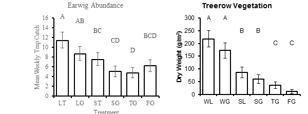
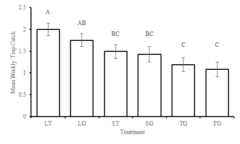
This is the most simple version of my model and it already seams over-parameterized (if I am using that term correctly). The next step I would like to do is add the continuous variable 'vegetation' which is an index of habitat vegetation that was sampled at the site of insect trapping. It is a smaller data-set because I sampled insects much more frequently than vegetation. I have run the same model on the vegetation data using transformations and the results were highly significant. Of the six treatments, 2 yield very little vegetation, 2 medium, and 2 that are very high. The insect data responded similarly but was less significant in the analysis. A comparison is below. How would one address the effect of vegetation on abundance? Simple linear regression (plotting mean earwigs by mean vegetation per month) is a very mess graph.

Thank you any and all for any and all help! I meet with my stats advisor again next week, I hope to present to her a working 'dist=Keyword' model.

Cheers,

Andrew

[SteveDenham]

Hey Andrew,

There is a lot going on here, so if I address a small part first and that helps, then we can go on to more stuff.

The thing about the chosen transformation (square root) is that it isn't available as a default in GLIMMIX.  You can program around it and all, but there is no distribution available for which the square root is the canonical link.  So, that just kind of stands there as a method that has been used in the entomology literature at least since the 1930's as a variance stabilizing transformation.

The example distribution that you specified was a negative binomial.  One thing that happens with R side models (residual option in the random statement for repeated effects) is that it leads to biased results when the distribution is one where the mean and variance are functionally related.  Examples are binomial, Poisson, and negative binomial.  Try re-running this:

proc glimmix data= earwig_2 method=laplace; /*Method more suitable for G side effects */

  plots=(studentpanel boxplot(fixed random  marginal  conditional  observed));

  class block  Cultivar Trt_Name Year DD_Mean;

  model Total_Earwigs=  Trt_Name | Year | DD_Mean/dist=nb ;

    random intercept Trt_Name / subject=Block(Cultivar Year);/* I think the actual repeated measures are on this subject by trt_name, and I prefer the AR + random effect model*/

  random DD_Mean / subject= Trt_Name*Year*Block(Cultivar) type=ar(1) ;

run;

/*

  lsmeans Trt_Name / diff adjust=tukey;

  lsmeans Trt_Name / pdiff lines;

    lsmeans DD_Mean;

    lsmeans Year;

    lsmeans Trt_Name*Year / plot=meanplot(join sliceby=Year cl) alpha=0.18 slice=Trt_Name;

  lsmeans Trt_Name*DD_Mean / plots=meanplot(join sliceby=DD_Mean cl) alpha=0.18;

  lsmeans Trt_Name*DD_Mean / plots=meanplot(join sliceby=Trt_Name cl) alpha=0.18;

  lsmeans DD_Mean*Year / plots=meanplot(join sliceby=Year cl) alpha=0.18 slice=DD_Mean;

    run;*/

I commented out the lsmeans for now, to concentrate on the model fitting (although I do want to come back and ask why an alpha of 0.18).

We can address the effect of vegetation as a covariate if we can get this part of the situation addressed first.

Steve Denham

[Hornet1937]

Thank you Steve! Sorry if I am over-complicating matters. I like this approach of one step at a time.

This model is working better. The type III tests of fixed effects were significant. Year*Trt_name was the only effect that had been significant in the transformation model that was not in the nb model. Is this because of the random statement " random intercept Trt_Name / subject=Block(Cultivar Year);"? The intercept statements have always confused me. I understand the next line,   random DD_Mean / subject= Trt_Name*Year*Block(Cultivar) type=ar(1) ; states that on each DD_Mean (date) I sampled trt_name with-in a given year, within a given cultivar, within a given block. But I would interpret the former statement to mean that I changed which treatment was in each plot each year? That is not the case, so I am probably mistaken. Also, you mentioned here and in other posts that you prefer the AR + Random effects model, how exactly is that implemented? "type=Ar(1)+VC"?

Moving along, I only chose NB because I have read that that is what most insect samples follow. Should I try out different ones and compare the fit statistics? I tried a poisson dist model and the AIC didn't change much.

Finally, I turned the lsmeans statements back on to get the T grouping. The results were similar to the transformed model but with less separations of treatments SG and TG. I don't remember why I was told to use an alpha of 0.18, I vaguely recall my adviser say that it was because the criteria is being partitioned between something or for adjusting for multiple tests. I will ask when I meet with them next. Would you recommend that I revert to the standard .05 in the interim?

Again, thank you for your much-needed help. I've aced every stats class that I've taken but still feel inept. They don't teach GLMMs in general courses.

Cheers,

Drew

[SteveDenham]

First question: Is this because...?  My answer: Probably.  Getting the right error term is critical.  This statement says that there are two variance components to consider, due to the design.  The first is block*cultivar*year and the second is trt_name*block*cultivar*year.  You multiply the subject through the "before slash" terms.  Using the subject= syntax imporves performance.

Second question: This specification should make it clear that this is the AR + Random effect model.  The subject to the repeated G side model is also a term in the random effects.  See Littell et al. in the Journal of Animal Science (1998) 72:1216.

Third question: I would look at the Poisson distribution as well, using AICC to compare.  Also check the overdispersion ratio (chi square to df) in the fit stats.  It should be near one.

Fourth question: We can address multiple comparisons a lot of ways.  The more I think of it, the 0.18 probably comes out of Tukey's method for the number of comparisons available, so that the lines option actually matches up with the adjusted p values.

Get a copy of Walt Stroups's Generalized Linear Mixed Models.  The preface says that hardest thing about GLMM's is "un-teaching" all of the things learned in the general courses.  And I am starting to get it.

Steve Denham