Glimmix - What distribution to use? Data appears to follow a leptokurtic distribution?

[DelBS]

Hi,

I'm second-guessing my GLIMMIX model and I'm wondering if anybody can chime in as to whether I selected the correct distribution and covariance structure. If you are willing please have a look and let me know if what I've done seems correct or if I should have proceeded differently at any point. I am no expert, but am I correct to think that a leptokurtic  distribution is more appropriate? Is that possible in glimmix?

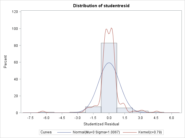
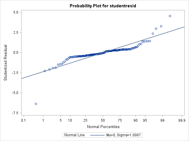
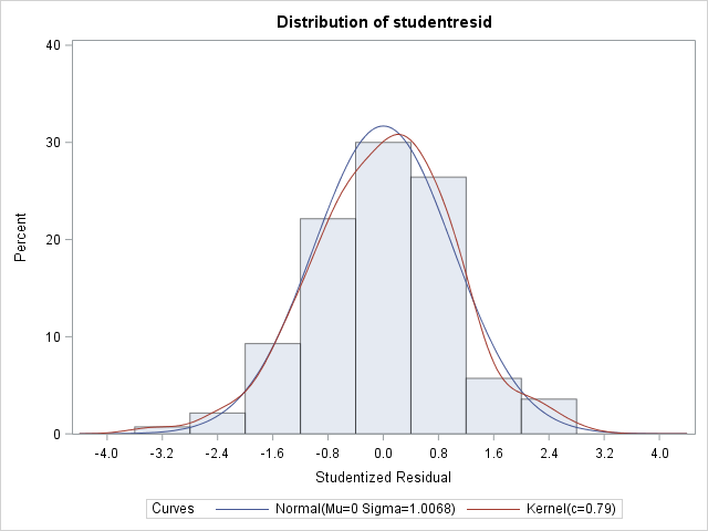
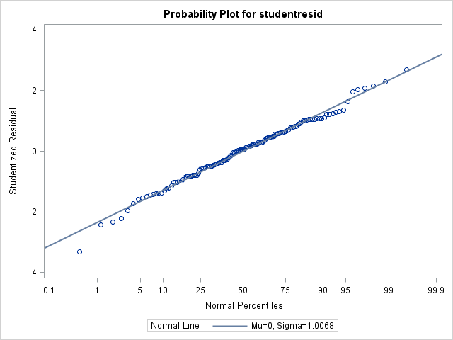
1) To start, here is what my data looks like with default normal distribution and identity link, without covariance structure. At this point, the residual plots show a lot of heterogeneity over my two fixed factors.1841.53 at this point.

Proc glimmix data=final;
class block peptide conc;
model fluo= peptide|conc / ddfm=kr;
random block;

Moments 
N 140 Sum Weights 140 
Mean 0 Sum Observations 0 
Std Deviation 1.00673643 Variance 1.01351824 
Skewness -0.8307546 Kurtosis 14.5027557 
Uncorrected SS 140.879035 Corrected SS 140.879035 
Coeff Variation . Std Error Mean 0.08508476 

Tests for Normality 
Test Statistic p Value 
Shapiro-Wilk W 0.775145 Pr < W <0.0001 
Kolmogorov-Smirnov D 0.194533 Pr > D <0.0100 
Cramer-von Mises W-Sq 1.403591 Pr > W-Sq <0.0050 
Anderson-Darling A-Sq 7.83746 Pr > A-Sq <0.0050 

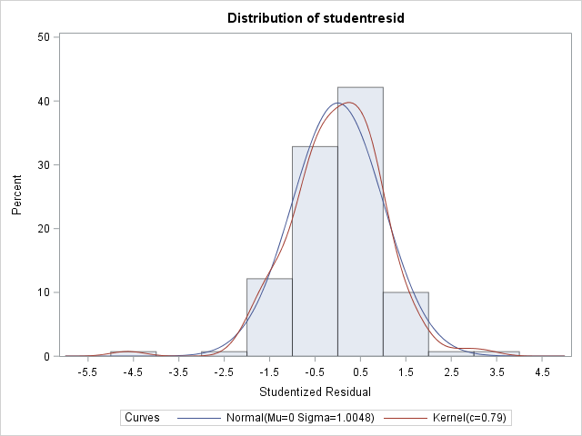
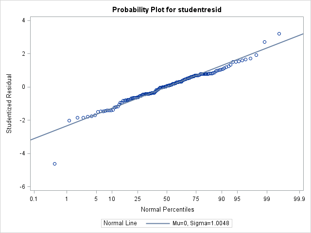
2) My stats professor (without having actually looked at my data, only experimental design) suggested a lognormal distribution. Here is what my data looks like when I used dist=lognormal link=identity in my model statement. The AICC fit statistic is improved to 58.88 with this change, and there are no longer any obvious heterogeneity over factor levels apparent in the residual plots.

Proc glimmix data=final;
class block peptide conc;
model fluo= peptide|conc / distribution=lognormal link=identity ddfm=kr;
random block;

Moments 
N 140 Sum Weights 140 
Mean 0 Sum Observations 0 
Std Deviation 1.00483965 Variance 1.00970273 
Skewness -0.4700973 Kurtosis 2.89471718 
Uncorrected SS 140.348679 Corrected SS 140.348679 
Coeff Variation . Std Error Mean 0.08492445 

Tests for Normality 
Test Statistic p Value 
Shapiro-Wilk W 0.964833 Pr < W 0.0011 
Kolmogorov-Smirnov D 0.065207 Pr > D 0.1494 
Cramer-von Mises W-Sq 0.09275 Pr > W-Sq 0.1420 
Anderson-Darling A-Sq 0.680749 Pr > A-Sq 0.0779 

3) Because the assumption of normality was not met, my textbook advised to try using a covariance structure for heterogeneous error. Is this appropriate even though dist=lognormal eliminated obvious signs of heterogeneity in the residual plots?  Doing so over one of my fixed effects improved the AICC from 58.88 to 56.74, and as well normality was met whereas it wasn't without the covariance structure

Proc glimmix data=final;
class block peptide conc;
model fluo= peptide|conc / distribution=lognormal link=identity ddfm=kr;
random block;
random _residual_ / subject=block*peptide*conc group=conc;

Moments 
N 140 Sum Weights 140 
Mean 0 Sum Observations 0 
Std Deviation 1.00680378 Variance 1.01365386 
Skewness -0.2048229 Kurtosis 0.48666309 
Uncorrected SS 140.897887 Corrected SS 140.897887 
Coeff Variation . Std Error Mean 0.08509045 

Tests for Normality 
Test Statistic p Value 
Shapiro-Wilk W 0.991907 Pr < W 0.6061 
Kolmogorov-Smirnov D 0.04681 Pr > D >0.1500 
Cramer-von Mises W-Sq 0.043249 Pr > W-Sq >0.2500 
Anderson-Darling A-Sq 0.314874 Pr > A-Sq >0.2500 

Thanks for the input