- Home
- /
- Programming
- /
- SAS Procedures
- /
- Glimmix for ordinal data
- RSS Feed
- Mark Topic as New
- Mark Topic as Read
- Float this Topic for Current User
- Bookmark
- Subscribe
- Mute
- Printer Friendly Page
- Mark as New
- Bookmark
- Subscribe
- Mute
- RSS Feed
- Permalink
- Report Inappropriate Content
Hi,
I am building a ordinal(probit) mixed model for ordinal data. My code looks as shown below. For the purpose of comparison with an proc nlmixed model, I want to set the intercept of the first category to 0. Is this possible with proc glimmix? In addition, I still want to model probabilities of a higher internet value.
proc glimmix data=k.golven_long method=quad(qpoints=5) ;
parms (1.2061);
class internet id;
model internet = time/ dist=multinomial link=CPROBIT solution;
random int/type=un subject=id ;
run;
Thanks in advance,
Margaux
- Mark as New
- Bookmark
- Subscribe
- Mute
- RSS Feed
- Permalink
- Report Inappropriate Content
The PROC GLMIMMIX doc includes a section on response-level order and how to choose a reference level. Most of the details are in the doc for the LOGISTIC procedure.
If you want to model probabilities of the highest value, I suggest using REF=LAST or EVENT='highestvalue', where highestvalue is the highest value for the INTERNET variable.
I guess I am confused by your request to "set the intercept of the first category to 0." When you use REF=LAST, you are setting the parameters for the last category, not the first. After you choose the reference response value, the other parameter estimates are determined by the data. You can use the NOINT option on the MODEL statement to suppress the intercept term for the entire model. Can you give an example of what you are trying to do?
- Mark as New
- Bookmark
- Subscribe
- Mute
- RSS Feed
- Permalink
- Report Inappropriate Content
Thank you for your quick response.
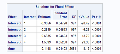
I want to fix the intercept of internet=1 to 0. In addition, I want the intercept of internet=5 to be estimated. Underneath you can find an example of the code I tried out and the obtained results.
proc glimmix data=k.data2 method=quad(qpoints=5) ;
parms (1.2061);
class internet(REF=first) id ;
model internet = time/ dist=multinomial link=CPROBIT solution;
random int/type=un subject=id ;
run;
- Mark as New
- Bookmark
- Subscribe
- Mute
- RSS Feed
- Permalink
- Report Inappropriate Content
I can't replicate this apparent problem when I use PROC GLIMMIX. When I use REF=FIRST or REF=LAST, it works as expected.
I point out that the models are identical whether you use REF=FIRST or REF=LAST or if there is some bug that causes the output you show. The effect of each of the Internet levels is identical when you use algebra to add in the intercept yourself. I wrote a brief explanation of this for a simpler case — see Re: Interpreting Multivariate Linear Regression with Categorical Varia... - SAS Support Communities, an example that also applies to your INTERNET variable.
If you run this code on data set SASHELP.CARS to have SAS do the algebra, you will see that the effect of each level of CYLINDERS (which plays the same role as your variable INTERNET) for Origin='Europe' is the same after you do the algebra (and it would be the same for Origin='USA' or for Origin='Asia').
proc glimmix data=sashelp.cars(where=(type='Sports'));
ods output parameterestimates=parms1;
nloptions gconv=0.01;
class cylinders(ref=first);
model origin = cylinders msrp / dist=multinomial solution;
run;

proc glimmix data=sashelp.cars(where=(type='Sports'));
ods output parameterestimates=parms2;
class cylinders(ref=last);
model origin = cylinders msrp / dist=multinomial solution;
nloptions gconv=0.01;
run;

proc sort data=parms1;
    by effect origin cylinders;
run;
proc sort data=parms2;
    by effect origin cylinders;
run;

data combine;
    merge parms1 parms2(keep=estimate rename=(estimate=estimate2));
    if effect='Cylinders' then do;
        adj_europe1=estimate+4.02179167; /* 4.02179167 is the intercept for Europe when REF=FIRST */
        adj_europe2=estimate2+1.00378568; /* 1.00378568 is the intercept for Europe when REF=LAST */
    end;
run;
Paige Miller
- Mark as New
- Bookmark
- Subscribe
- Mute
- RSS Feed
- Permalink
- Report Inappropriate Content
I assume you mistakenly think that my covariate is of ordinal nature. It is however my response that is of ordinal nature.
In the sashelp model and code, origin plays the role of the internet variable in my data. Notice how also the last category (USA) has no threshold (called intercept by SAS) estimate, while the other categories do.
The model that I am applying is explained in the following paper of Hedeker and Gibbons (1994): https://www.jstor.org/stable/2533433. They set the first threshold (called 'intercept' by SAS software) at 0.
- Mark as New
- Bookmark
- Subscribe
- Mute
- RSS Feed
- Permalink
- Report Inappropriate Content
The concept remains the same whenever you have categorical predictor variables. The model is the same, the fit is the same, the predicted values are the same, the coefficients are the same after you do the algebra; but you get different parameterizations of the model depending of REF=FIRST or REF=LAST or REF=something_else. Ordinal or nominal response is not relevant to this issue of how the model is paramterized and how the model is the same after you do the algebra.
Paige Miller
- Mark as New
- Bookmark
- Subscribe
- Mute
- RSS Feed
- Permalink
- Report Inappropriate Content
Ok, I think I know the problem why REF=FIRST and REF=LAST is not working for you.
The CLASS statement is for predictor variables only, not for response variables. So your INTERNET variable is a response variable and thus the CLASS statement has no impact.
If you want the REF=FIRST or REF=LAST to apply to the response variable, you can do this in the MODEL statement.
model internet (ref=last) = ...
The idea that the model is the same, even though the parameterization is different, still holds.
Paige Miller
- Mark as New
- Bookmark
- Subscribe
- Mute
- RSS Feed
- Permalink
- Report Inappropriate Content
I have tried that, but to no avail.
- Mark as New
- Bookmark
- Subscribe
- Mute
- RSS Feed
- Permalink
- Report Inappropriate Content
@PaigeMiller wrote:
If you want the REF=FIRST or REF=LAST to apply to the response variable, you can do this in the MODEL statement.
Yes, the links that I provided are for how to control the order of the RESPONSE variable, not explanatory variables.
Note: the links that I provided show how to control the order of the RESPONSE variable. Here are the links again:
The PROC GLMIMMIX doc includes a section on response-level order and how to choose a reference level. Most of the details are in the doc for the LOGISTIC procedure.
Catch up on SAS Innovate 2026
Dive into keynotes, announcements and breakthroughs on demand.
Explore Now →Learn the difference between classical and Bayesian statistical approaches and see a few PROC examples to perform Bayesian analysis in this video.
Find more tutorials on the SAS Users YouTube channel.
SAS Training: Just a Click Away
Ready to level-up your skills? Choose your own adventure.


