debug a subroutine; Call NLPQN

[Salah]

Hello

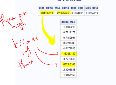
I am using (call nlpqn) in order to find MLEs. What I noticed is that the bias is extremely high for some data sets but not all of them. I don't know why this is happening? 

So I tried to debug the subroutine by adding a print statement inside the subroutine to found that there are normal or close values of my likelihood function followed by spikes then values go back to normal values. If I increase the number of the simulation then I get more of these spikes!!!

Any clue why this is happening?

Thank you

proc iml;

n=20;

m=10;

R=J(m, 1, 0);

R[1]=10;

seed=22;

k=10;

alpha=1.5;

beta=0.8;

***********************************************************************************************;
*** LOG likelihood for the Lomax using Type II Adaptive progressive censoring ***** ;
***********************************************************************************************;

start log_func(y) global (n,m,X,R,q);

func=0;

alpha=y[1];
beta=y[2];

Rq=R[1:q];

Sum1=0;
Do i=1 to m;
Sum1=sum1+log(1+beta*X[i]);
end;

Sum2=0;
Do i=1 to q;
Sum2=Sum2+R[i]*log(1+beta*X[i]);
end;

func=func+m*log(alpha*beta)-(alpha+1)*Sum1-alpha*sum2-alpha*(n-m-Rq[+])*log(1+beta*X[m]);

*print func;

Return(func);

finish;

******************************************************************************************;
alpha_MLE=J(k,1,0);beta_MLE=J(k,1,0); MSE_a=J(k,1,0); MSE_b=J(k,1,0);

Do N1=1 to K;

****     Simulation       ***;
****************************;

W=J(m,1,0);V=J(m,1,0);U=J(m,1,0); X_p=J(m,1,0); X_A=J(m,1,0); X=J(m,1,0);

do i=1 to m;
W[i]=Uniform(seed);
end;

S=1+R[m];
V[1]=W[1]**(1/S);

do i=2 to m;
S=S+(1+R[m-i+1]);
V[i]=W[i]**(1/S);
end;

do i=1 to m;

U[i]=1-prod( V[ m:( m-i+1)] );** the U's are the required progressively type II from U(0,1);

END;

**********************;

Call sort (U);
X_p=( (1-U)##(-1/alpha) -1 )/beta;

call sort (X_p);

*T= X_p[m/2];

*T=X_p[4*m/5];

T=X_p[m]+2;

do idx=1 to m-1;
if (( X_p[idx] < T) & (X_p[idx+1] >= T)) then q=idx;
end;

If X_p[m]>T then

do;

X_1_q=J(q,1,0);

X_1_q= X_p[1:q]; /* extract those failures that are less than T i.e. all X_1,...,X_j,X_(j+1) */

Xp_remaining=J(m-q,m,0); Y=J(m-q,m,0);

Y=X_p[q+1:m];

**************************************************;
** Generate data of size m-q **;
**************************************************;
W1=J(m-q,1,0);  YY=J(m-q,1,0); 

***************************************************************;
call randseed(seed);
call randgen(W1, "Uniform",0,1);

Call sort (W1);

YY=( (1-W1)##(-1/alpha)#(1+beta*T)-1 )/beta;

X_A= X_1_q //YY;

X=X_A;

end; 

else if ( X_p[m] <= T) then

do;
q= m;
X = X_p;

end; 

************* Constrain***********************;

con={.0001 .0001 , . .};
opt={1};
x0={0,0};

*************** MLE *********************;
tc={8000 12000};

call nlpqn(rc, y_ret, "log_func", x0, opt, con,tc);

alpha_mle[N1]=y_ret[1];
beta_mle[N1]=y_ret[2];

MSE_a[N1]=(alpha_mle[N1]-alpha)**2;
MSE_b[N1]=(beta_mle[N1]-beta)**2;

END; *end simulation;

Bias_alpha=abs(alpha_MLE[:]-alpha);

Bias_beta=abs(beta_MLE[:]-beta);

MSE_alpha=MSE_a[:]/m;
MSE_beta=MSE_b[:]/m;

print Bias_alpha MSE_alpha Bias_beta MSE_beta ;

print alpha_mle;

quit;

[Rick_SAS]

I am out of the office this week, so I can't run your program. However, it looks like your initial guess is (0,0), which violates the constraints. Try using a different initial guess, such as (1,1).

Another possibility for "spikes" are singularities on the loglikelihood function, which involves the term log(1+beta*X[i]);  Of the LL might not have a local extremum. My suggestion: Find a data set that is showing the problem. Graph the LL(alpha, beta) as a function of (alpha,beta) on the interval (0.001,10] x (0.001,10] to get a feeling for the graph of the LL on the domain.

To graph the LL, you can evaluate the LL on a dense grid of points and use a scatter plot and the COLORERESPONSE= option. See https://blogs.sas.com/content/iml/2016/07/18/color-markers-third-variable-sas.html 

[Salah]

I did what you suggested, unfortunately, I got  "ERROR: Variable OPTION not found"

In case the code worked then what? I am not sure about what I will find? Should I be able to see if there is a local maximum? 

proc iml;

n=25; m=15; R=J(m, 1, 0); R[1]=10;

seed=0; k=10;

alpha=1.5; beta=0.8;

*** generate a grid of points **;
********************************;

/* varies SLOW <-----------------> FAST */
/* values for alpha beta */

k = expandgrid(0.001:10, 0.001:10 );

start Func(Z) global (n,m,X,R,q);

Sum1=0;
Do i=1 to m;
Sum1=sum1+log(1+z[,2]*X[i]);
end;

Sum2=0;
Do i=1 to q;
Sum2=Sum2+R[i]*log(1+z[,2]*X[i]);
end;

Rq=R[1:q];

LL=m#log(z[,1]#z[,2])-(z[,1]+1)#Sum1-z[,1]#sum2-z[,1]#(n-m-Rq[+])#log(1+z[,2]#X[m]);

return( LL);

finish;

********************************************************************************************;
** progressive censoring ***;
****************************;

W=J(m,1,0);V=J(m,1,0);X_p=J(m,1,0); X_A=J(m,1,0); U=J(m,1,0);

X=J(m,1,0);

do i=1 to m;
W[i]=Uniform(seed);
end;

S=1+R[m];
V[1]=W[1]**(1/S);

do i=2 to m;
S=S+(1+R[m-i+1]);
V[i]=W[i]**(1/S);
end;

do i=1 to m;

U[i]=1-prod( V[ m:( m-i+1)] );

END;

**********************;

Call sort (U);

X_p=( (1-U)##(-1/alpha) -1 )/beta;

call sort (X_p);

*T= X_p[m/2];

*T=X_p[4*m/5];

T=X_p[m]+2;

do idx=1 to m-1;
if (( X_p[idx] < T) & (X_p[idx+1] > T)) then q=idx;
end;

If X_p[m]>T then

do;

X_1_q=J(q,1,0);

X_1_q= X_p[1:q];

Xp_remaining=J(m-q,m,0); Y=J(m-q,m,0);

Y=X_p[q+1:m];

**************************************************;
** Generate data of size m-q **;
**************************************************;

W1=J(m-q,1,0); YY=J(m-q,1,0);

call randseed(seed);

call randgen(W1, "Uniform",0,1);

Call sort (W1);

YY=( (1-W1)##(-1/alpha)#(1+beta*T)-1 )/beta;


X_A= X_1_q //YY;

X=X_A;

end;

else if ( X_p[m] <= T) then

do;
q= m;
X = X_p;

end;

f = Func(k);

print k[c={"alpha" "beta" }] f;

alpha=K[,1]; Beta=K[,2];

create _Temp var {alpha, beta};
append;
close _Temp;

submit;
title "Graph log-Likelihood function";
proc sgplot data=_Temp;
scatter x=alpha y=beta / colorresponse=option
markerattrs=(symbol=CircleFilled size=14); /* big filled markers */
run;

endsubmit;

quit;

[IanWakeling]

The error message is telling you that the variable called "option" does not exist in the data set _Temp.  You need to export the LL to this data set by adding "f" to the variable list in the CREATE statement and, then use colorresponse=f.

[Rick_SAS · Accepted solution]

1. You probably need a denser grid. Maybe something like

xrange = 0.001 || do(0.1, 5, 0.1);

yange = x;

k = expandgrid( xrange, yrange );

2. You are trying to visualize the LL, so you need to write the 'f' value as well:
create _Temp var {alpha beta f};
append;
close _Temp;

3. Use COLORERESPONSE=f

4.My suggestion is the first item in the list of 10 tips before you run an optimization. The other tips might also be helpful. I think you are doing some of them.

5. In case the code worked then what? I am not sure about what I will find? Should I be able to see if there is a local maximum? 
Yes, the idea is that this enables you to visualize the LL for the cases that are failing. It should help you figure out the next step.

[Salah]

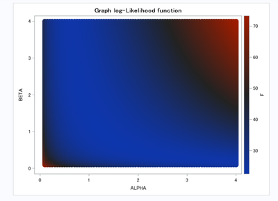
The code is working with no errors but I am confused regarding the outcome values and the graph.

each time I change the range of my parameters I get different initial values

for example if I choose KK = ExpandGrid( do(0.001,10,0.05), do(0.001,10,.05) ); then the values that maximize LL are (alpha, beta)= (9.95, 9.95), for KK = ExpandGrid( do(0.001,2,0.05), do(0.001,2,.05) ) I get  (alpha, beta)= (0.001, 0.001), for KK = ExpandGrid( do(0.1,4,0.05), do(0.1,4,.05) );  I get (4,4) and so on. I am not sure what range should work?

Moreover, the graph looks confusing. 

I should look at the red spot that indicates a maximum LL .....correct??

I thought that there will be a trend like what I saw in the blogs, instead, I saw things like this  with no trend

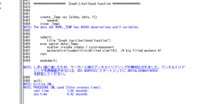
The last thing I may need help with is why all of the sudden I start to have things written in Chinese in the log file!!!!! I don't recall doing anything I was just trying to play with the range of my parameters. 

The modified code:

proc iml;

n=25; m=15; R=J(m, 1, 0); R[1]=10;

seed=0; k=10;

alpha=1.5; beta=0.8;

********************************************************************************************;
** progressive censoring ***;
****************************;

W=J(m,1,0);V=J(m,1,0);X_p=J(m,1,0); X_A=J(m,1,0); U=J(m,1,0);

X=J(m,1,0);

do i=1 to m;
W[i]=Uniform(seed);
end;

S=1+R[m];
V[1]=W[1]**(1/S);

do i=2 to m;
S=S+(1+R[m-i+1]);
V[i]=W[i]**(1/S);
end;

do i=1 to m;

U[i]=1-prod( V[ m:( m-i+1)] );

END;

**********************;

Call sort (U);

X_p=( (1-U)##(-1/alpha) -1 )/beta;

call sort (X_p);

T= X_p[m/2];

*T=X_p[4*m/5];

*T=X_p[m]+2;

do idx=1 to m-1;
if (( X_p[idx] < T) & (X_p[idx+1] >= T)) then q=idx;
end;

If X_p[m]>T then

do;

X_1_q=J(q,1,0);

X_1_q= X_p[1:q];

Xp_remaining=J(m-q,m,0); Y=J(m-q,m,0);

Y=X_p[q+1:m];

**************************************************;
** Generate data of size m-q **;
**************************************************;

W1=J(m-q,1,0); YY=J(m-q,1,0);

call randseed(seed);

call randgen(W1, "Uniform",0,1);

Call sort (W1);

YY=( (1-W1)##(-1/alpha)#(1+beta*T)-1 )/beta;


X_A= X_1_q //YY;

X=X_A;

end;

else if ( X_p[m] <= T) then

do;
q= m;
X = X_p;

end;

/* four-hump camel has two global maxima:
p1 = {-0.08984201 0.71265640 };
p2 = { 0.08984201 -0.71265640 }; */

start Camel(KK) global (n,m,X,R,q);

alpha = KK[,1]; beta = KK[,2];

Rq=R[1:q];

Sum1=0;
Do i=1 to m;
Sum1=sum1+log(1+beta*X[i]);
end;

Sum2=0;
Do i=1 to q;
Sum2=Sum2+R[i]*log(1+beta*X[i]);
end;

f=m#log(alpha#beta)-(alpha+1)#Sum1-alpha#sum2-alpha#(n-m-Rq[+])#log(1+beta#X[m]);


return( -f ); /* return -f so that extrema are maxima */
finish;

KK = ExpandGrid( do(0.1,4,0.05), do(0.1,4,.05) );

f = Camel(KK);

optIndex = loc(f=max(f)); /* find maximum values of z */
opt_parameter = KK[optIndex,]; /* corresponding (alpha,beta) values */

print opt_parameter;

*print q x kk[c={"alpha" "beta" }] f ;

alpha=Kk[,1]; Beta=Kk[,2];

******************* Graph Likelihood function ****************;

create _Temp var {alpha, beta, f};
append;
close _Temp;

submit;
title "Graph log-Likelihood function";
proc sgplot data=_Temp;
scatter x=alpha y=beta / colorresponse=f
markerattrs=(symbol=CircleFilled size=14); /* big filled markers */
run;

endsubmit;

quit;

[Rick_SAS]

I am out of the office this week, so the best I can do is remind you that the LL depends on the data. You are using seed=0, so you get a DIFFERENT likelihood function every time you run your function. 

Use a positive seed value for reproducibility.

When you see a LL function where the red area is on the boundary, it probably means that the maximum is outside of the domain you are using for ExpandGrid. It might even mean that the function is unbounded. It appears that for some of your random data set, the model does not fit the data. These are the 'spikes' where the optimal (alpha,beta) values are much different than for the bulk of the other data sets. 

You either need to reexamine how you are generating the data (is your simulation correct?)  or you need to generate larger data sets so that the LL function has a well-defined maximum for most data sets.

I have no idea why you are getting Chinese characters. 

[FreelanceReinh]

---

@Salah wrote:

The last thing I may need help with is why all of the sudden I start to have things written in Chinese in the log file!!!!! I don't recall doing anything I was just trying to play with the range of my parameters.

---

Hello @Salah,

Thank you so much for bringing this up! I've always been wondering (with low priority, though) how to get rid of the rare, but consistently obtained German messages in my log files, typically from PROC SGPLOT and related procedures. Seeing the Japanese (?) note in your log screenshot I got the idea: Change the LOCALE= system option to EN_US.

options locale=EN_US;

My original setting was DE_DE and yours might be JA_JP.

Finally (after six years) my logs are all English! I'm really happy about this. Thanks again! 🙂

[Salah]

Thank you so much. It works!!!
I didn't know that PROC SGPLOT caused the shift of the language in the log file!!!
WOOOW I learn a new thing today. Thanks a lot!!!!