SAS Miner Clustering options

[BenDSW]

Hi SAS-folks,

I have been playing around with SAS Miner and focused on the clustering part as I want to understand the possibilities.

So far, I have been able to answer various questions regarding clustering in SAS, but I have not yet been able to answer the following questions:

1. Is it possible to use a different distance metric than Euclidean distance? For example, manhattan/cityblock, cosine, and so on. Some of these are available in SAS/STAT with the appropriate proc clusters. So far I have only found I can choose 'ward', 'average' and 'centroid'.

2. Is it possible to provide my own initialization for the clustering? For example, picking instances myself, or utilize a different algorithm (implemented SAS/base or SAS/Miner)?

3. Is it possible to cluster new observations using a found clustering model? E.g. I first cluster with a subset of my data, find a number of clusters and then I want to assign the observations in the remaining data to these clusters?

4. And most importantly, I wish to find more information about what everything does in SAS/Miner. I have been looking around on the internet for hours and have yet to find a more detailed explanation of everything than the level of '4-word descriptions per attribute'. For example, in SAS/Miner the explanation for CCC Cutoff is "Cubic clustering criterion cutoff".

Thanks in advance,

Sincerely,

Ben

[M_Maldonado · Accepted solution]

Hi Ben,

Thanks for your detailed questions!

1. The three clustering methods you mention are the only ones supported on Enterprise Miner.

2. On Enterprise Miner you can specify a few seed initialization methods for the cluster node. But if you are looking to point a proc to a specific data set, you should use proc fastclus with the seed option ().

3. A quick way to cluster new observations is to run a cluster node on the subset of your data, and then use that flow to score a new data set (with a score role).

4. The best place to find detailed explanations is right on Enterprise Miner. Go to the contents icon, or press F1. This will open the reference help.

For example, I punched F1 on EM and searched for "Cubic clustering criterion". I got more than 25 pages of detailed explanation... Brief excerpt below of the abstract and intro.

I hope this helps for now.

Thanks,

Miguel

Cubic Clustering Criterion

---

Abstract

The cubic clustering criterion (CCC) can be used to estimate the number of clusters using Ward's minimum variance method, k -means, or other methods based on minimizing the within-cluster sum of squares. The performance of the CCC is evaluated by Monte Carlo methods.

---

Introduction

The most widely used optimization criterion for disjoint clusters of observations is known as the within-cluster sum of squares, WSS, error sum of squares, ESS, residual sum of squares, least squares, (minimum) squared error, (minimum) variance, (sum of) squared (Euclidean) distances, trace(W), (proportion of) variance accounted for, or R² (see, for example, Anderberg 1973; Duran and Odell 1974; Everitt 1980). The following notation is used herein to define this criterion:

n

number of observations

n_k

number of observations in the k^th cluster

p

number of variables

q

number of clusters

X

n by p data matrix

q by p matrix of cluster means

Z

cluster indicator matrix with element Z_ik = 1 if the i^th observation belongs to the k^th cluster, 0 otherwise.

Assume that without loss of generality each variable has mean zero. Note that Z'Z is a diagonal matrix containing the n_ks and that

The total-sample sum-of-squares and cross products (SSCP) matrix is

T = X’X.

The between-cluster SCCP matrix is

The within-cluster SSCP matrix is

The within-cluster sum of squares pooled over variables is thus trace(W). By changing the order of the summations, it can also be shown that trace(W) equals the sum of squared Euclidean distances from each observation to its cluster mean.

Since T is constant for a given sample, minimizing trace(W) is equivalent to maximizing

which has the usual interpretation of the proportion of variance accounted for by the clusters. R² can also be obtained by multiple regression if the columns of x are stacked on top of each other to form an np by 1 vector, and this vector is regressed on the Kronecker product of z with an order p identity matrix.

Many algorithms have been proposed for maximizing [untitled graphic] or equivalent criteria (for example, Ward 1963; Edwards and Cavalli-Sforza 1965; MacQueen 1967; Gordon and Henderson 1977). This report concentrates on Ward's method as implemented in the CLUSTER procedure. Similar results should be obtained with other algorithms, such as the k-means method provided by FASTCLUS.

The most difficult problem in cluster analysis is how to determine the number of clusters. If you are using a goodness-of-fit criterion such as R², you would like to know the sampling distribution of the criterion to enable tests of cluster significance. Ordinary significance tests, such as analysis of variance F- tests, are not valid for testing differences between clusters. Since clustering methods attempt to maximize the separation between clusters, the assumptions of the usual significance tests, parametric or nonparametric, are drastically violated. For example, 25 samples of 100 observations from a single univariate normal distribution were each divided into two clusters by FASTCLUS. The median absolute t-statistic testing the difference between the cluster means was 13.7, with a range from 10.9 to 15.7. For a nominal significance level of 0.0001 under the usual, but invalid, assumptions, the critical value is 3.4, yielding an actual type 1 error rate close to 1.

The first step in devising a valid significance test for clusters is to specify the null and alternative hypotheses. For clustering methods based on distance matrices, a popular null hypothesis is that all permutations of the values in the distance matrix are equally likely (Ling 1973; Hubert 1974). Using this null hypothesis, you can do a permutation test or a rank test. The trouble with permutation hypothesis is that, with any real data, the null hypothesis is totally implausible even if the data does not contain clusters. Rejecting the null hypothesis does not provide any useful information (Huber and Baker 1977).

Another common null hypothesis is that the data are a random sample from a multivariate normal distribution (Wolfe 1970, 1978; Lee 1979). The multivariate normal null hypothesis is better than the permutation null hypothesis, but it is not satisfactory because there is typically a high probability of rejection if the data is sampled from a distribution with lower kurtosis than a normal distribution, such as a uniform distribution. The tables in Englemann and Hartigan (1969), for example, generally lead to rejection of the null hypothesis when the data is sampled from a uniform distribution.

Hartigan (1978) and Arnold (1979) discuss both normal and uniform null hypotheses, and the uniform null hypothesis seems preferable for most practical purposes. Hartigan (1978) has obtained asymptotic distributions for the within-cluster sum of squares criterion in one dimension for normal and uniform distributions. Hartigan's results require very large sample sizes, perhaps 100 times the number of clusters, and are, therefore, of limited practical use.

This report describes a rough approximation to the distribution of the R² criterion under the null hypothesis that the data have been sampled from a uniform distribution on a hyperbox (a p-dimensional right parallelepiped). This approximation is helpful in determining the best number of clusters for both univariate and multivariate data and with sample sizes down to 20 observations. The approximation to the expected value of R² is based on the assumption that the clusters are shaped approximately like hypercubes. In more than one dimension, this approximation tends to be conservative for a small number of clusters and slightly liberal for a very large number of clusters (about 25 or more in two dimensions). The cubic clustering criterion (CCC) is obtained by comparing the observed R² to the approximate expected R² using an approximate variance-stabilizing transformation. Positive values of the CCC mean that the obtained R² is greater than would be expected if sampling from a uniform distribution and therefore indicate the possible presence of clusters. Treating the CCC as a standard normal test statistic provides a crude test of the hypotheses:

H₀: the data has been sampled from a uniform distribution on a hyperbox.

H_a: the data has been sampled from a mixture of spherical multivariate normal distributions with equal variances and equal sampling probabilities.

Under this alternative hypothesis, R² is equivalent to the maximum likelihood criterion (Scott and Symons 1971).

[M_Maldonado]

Hi Ben,

To give you some more input.

1. The three clustering methods you mention are the only ones supported on Enterprise Miner.

2. On Enterprise Miner you can specify a few seed initialization methods for the cluster node. But if you are looking to point a proc to a specific data set, you should use proc fastclus with the seed option ().

3. A quick way to cluster new observations is to run a cluster node on the subset of your data, and then use that flow to score a new data set (with a score role).

I hope it is useful.

Good luck!

Miguel

[BenDSW]

Hi!

1. Ok thanks

2. So basically I can not provide my own initial points for clustering in SAS Miner?

3. I do not quite follow how I should proceed. I have tried a variety of setups. I think the one closest to your explanation is as follows:

subsetdata(role=raw) -> clustering -> score

alldata(role=score) -> score

but I do not obtain any results regarding 'this observation is clustered to cluster X' or something like that. What did you do assign clusters to a new data set using a found clustering model?

4. Thanks for the F1 suggestion, but I feel I require more info on certain parts, especially info on what is permissible/allowed for the data flows within the diagram.

[M_Maldonado]

Hi,

2. I don't know a lot about initialization, other than it is a crucial first step to find a good number of clusters. The initialization options in the cluster node (first, macqueen, principal components, and full/partial replacement) seem pretty data-driven to me. Is any of those similar to the initial points you would manually pass? How much value does it add if we surface an option to select initial points?

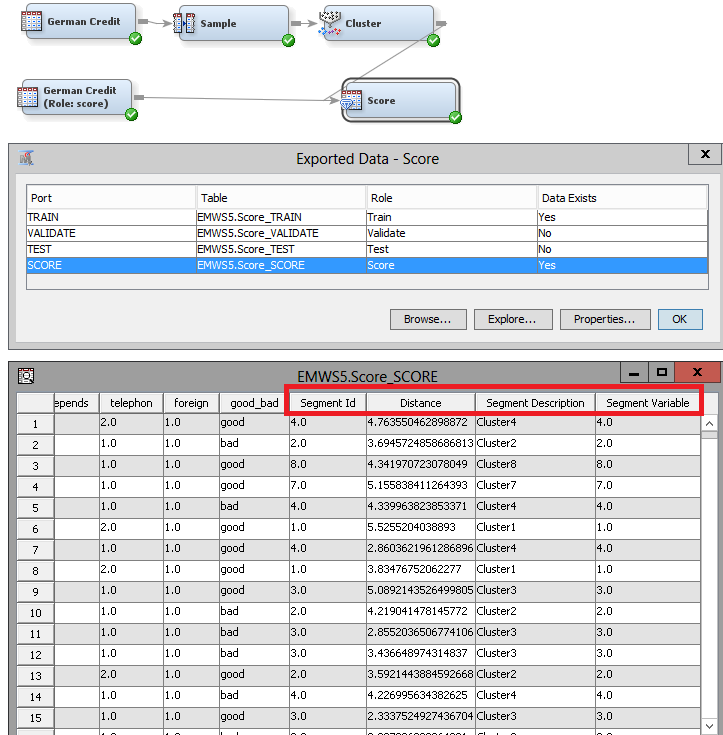
3. I think we have a similar flow. A screenshot below. Notice you can change the raw data source node or the score data source node for any other data sets. Once you run the flow, click on the ellipsis for Exported data of your Score node. Browse the score partition and notice the new columns in your data set: segment id, distance, segment description, and segment variable. The cluster node assigns metadata roles that make sense, so that you don't use redundant information on subsequent models.

If all you want to do is to find the clusters for a larger data set, you are good to go. If on the other hand, you want to use your large data set (the scored one) to train subsequent models (for example a model for each segment), you will need to add a SAS Code node and paste the below into the code editor. This code has two data steps. The first one creates a train data from your scored data set. The second one passes the metadata from your scored set.

data &EM_EXPORT_TRAIN;

set &EM_IMPORT_SCORE;

run;

data &EM_EXPORT_TRAIN_CMETA;

set &EM_IMPORT_SCORE_CMETA;

run;

4. I am not a programmer and it was relatively easy to pick up how SAS EM works. And just like the particular need you had for point 3, you can find a work around to do exactly what you want to do in SAS EM because it sits on top of base SAS. This means that 99% of the time, anything that you can do on base SAS you can do in EM. Something that really helped me understand EM was to go to my workspace folder (EMWS) and see what each node creates. When you run into trouble take a quick look to the "Getting started" section on the reference help, and feel free to post specific questions. Someone in this online community will point you in the right direction.

Thanks,

Miguel

[BenDSW]

Thanks a lot for the help!

3. So I was merely looking in the wrong fields for the output that I wanted.

2. As for initialization. This is pretty much the most important part of the K-means algorithm as it is prone to convergence to local optima. I feel it is imperative to specify the initialization myself. Although the ones in SAS Miner are decent, I much rather wish to use new(er) innovations such as K-means++ (see wikipedia).

4. Certainly, it is trivial to try every button/option out in SAS Miner and learn by playing, but I feel I am squandering a lot of time due to the vast amount of options and the general lack of correspondence to the machine learning terminology that I (and many others) are familiar with.

Thanks again!

[deemag]

Hi ,

Is there any way to do spacio,spacio temporal clustering in SAS EM?

Thanks much