Tip: Your First Time Series Forecasts with SAS® Enterprise Miner™

[#1]

If you are like most data miners, you generally work with cross-sectional data.  In a typical dataset, each observation represents a customer and the measurements (columns) collectively provide a snapshot of that customer at a particular point in time. You use traditional data mining and machine learning techniques to identify relationships among the variables and predict future outcomes.

When data are collected repeatedly over time, a special set of techniques known collectively as time series analysis is used to gain insight into patterns of change and to make predictions (forecasts) from historical values. Accurate forecasts are often critical for business planning—for example, they can help ensure appropriate staffing and inventory, taking into account the overall trend in the data as well as seasonal variations. 

Perhaps you have heard about time series analysis but it was not part of your formal training. Or maybe you've run across some time-stamped data and you want to know how to gain insight into it. This tip will help get you started with the time series and forecasting capabilities of Enterprise Miner.

Time Series Data

A time series is a sequence of measurements recorded at equally-spaced intervals (hourly, weekly, monthly, etc.). As the name suggests, time series are inherently temporal. They often exhibit trends or seasonal patterns.

For example, the following plot shows visits to a fitness center by month:

Fitness Center Visits By Month

Here, each data point represents the total number of individual visits to the fitness center. The number of visits was recorded monthly between 2002 and 2008.

What does the plot tell us? There doesn't appear to be an upward or downward trend in overall facility usage between 2002 and 2008. But the seasonal pattern is clear: visits tend to peak early in the year then decline through the summer months, followed by a big drop at the end of the year. This end-of-the-year drop and recovery in the following year are probably related to seasonal changes in behavior, as many of us get out of our normal fitness routine during the holiday months and resolve to get back into shape in the New Year.

This plot is pretty simple to produce. But because of the ‘equal interval’ restriction mentioned above, transactional data must be transformed before it can be used in a time series analysis. The following tables illustrate schematically how to transform transactional data into time series data.

Transaction ID	Date	Customer ID	Measure1	Measure2
1	January 1, 2002	1	5	1
2	January 5, 2002	2	2	1
3	February 25, 2002	1	10	1
4	March 12, 2002	3	6	1
5	March 25, 2002	3	8	1
…

Before: Transactional Data

Time	Time ID	Series1	Series2
1	January, 2002	7	2
2	February, 2002	10	1
3	March, 2002	14	2
…

After: Time Series

In this case date-stamped customer-level data are aggregated into monthly intervals using the sum of the values as the aggregation measure. The new series has a Time ID and two data series mapped from the Measure columns.

Generating Forecasts

Imagine that we have turned the clock back to early 2009 and we want to forecast fitness center utilization for the first half of the new year. Having accurate forecasts will help schedule sufficient staffing to meet our patrons’ needs, while avoiding costly overstaffing.

We can prepare the data and generate forecasts in Enterprise Miner with a simple three-node flow:

Data Source node

Here is a snippet of our historical data:

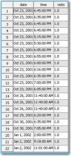
Input Data

Each row represents different date- and time-stamped visit to the fitness center. The number of visits is equal to 1 for every row because each row represents a single visit. 

The Data Source node defines modeling roles for the three columns:

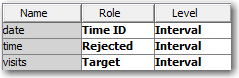
Variable roles

I’ve assigned Date as the TimeID and Visits as the target. Since our time interval is monthly, I’ve rejected the time of day variable. It is irrelevant.

TS Data Preparation node

The TS Data Preparation node transforms our data into a monthly series.

I’ve specified Month as desired the time interval and set Accumulation to Total. This will aggregate individual visits by month.

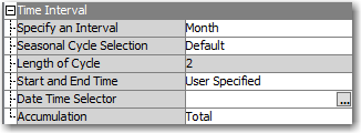
Time Interval Properties

To restrict the analysis to the time window of interest, ignoring early data points, I’ve specified a custom Start and End times for the series using the Date Time Selector control:

Start and End Times

When this node is run, the TS Data Preparation node exports the transformed dataset:

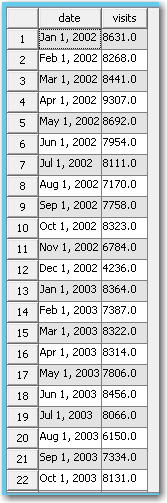
Exported Data

TS Exponential Smoothing node

Now to produce forecasts.

In Enterprise Miner, forecasting is supported using Exponential Smoothing, a very popular and useful method for producing forecasts.  This technique computes a new series of fitted values and forecasts, where each value in the series is the weighted average of the values observed at prior time points.  It is called "Exponential smoothing" because the weights decrease exponentially to ensure that recent observations carry more weight than older ones. Exponential Smoothing tends to work best for short-term forecasts, i.e., forecasting a few time periods into the future.

In node properties, I’ve accepted the default Forecasting Method (Automatic), which tells Enterprise Miner to try various exponential smoothing methods and choose the one that has the best fit to the observed series.

I’ve also set the Forecast Lead to 6, which will give us forecasts for the next 6 months.

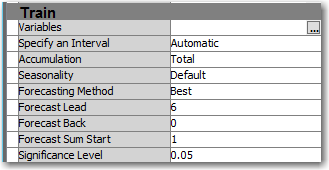
TSEM Node Properties

Results

Here is the plot of fitted values and forecasts that the TSEM node produces:

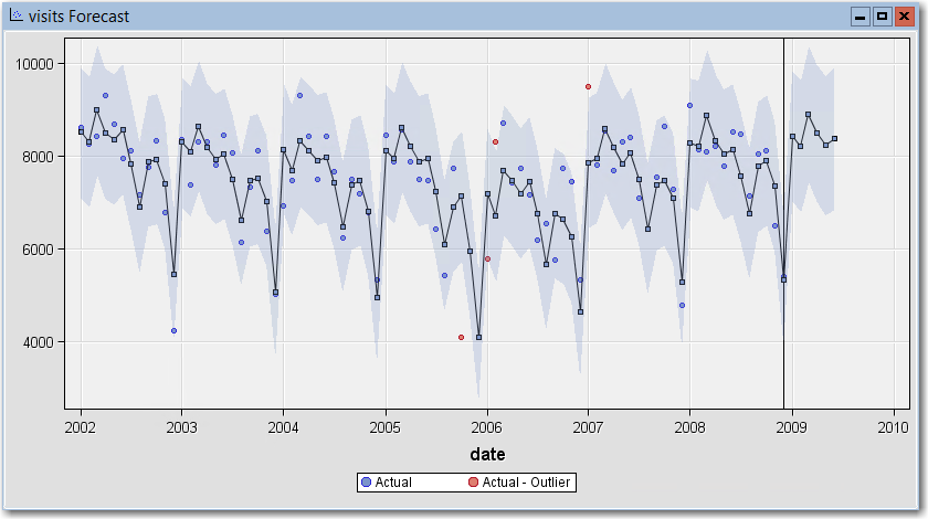
Forecast Plot

Actual number of visits are shown as blue dots. Smoothed (fitted) values appear as a line that overlays blue squares. The light blue band represents the confidence interval for the fitted values.

Exponential smoothing has picked up on the seasonal variations in our data. Within each year the smoothed values show an early spike in the number of visits followed a gradual decline.

By eyeballing the plot, you can gauge how well the smoothed values fit the observed values. But you can also refer to the Fit Statistics table (not shown here), which contains error-based fit measures like Mean Square Error and Mean Absolute Percent Error.

Forecasts and their confidence intervals appear to the right of the vertical reference line. Consistent with the seasonal pattern, the forecast calls for a rise in visits through March, then a drop off in subsequent months.

Conclusion

This tip has shown how prepare time-stamped data for time series analysis and to obtain demand forecasts for a fitness center. The steps were pretty simple:

1. Define your input datasource, TimeID, and Target.
2. Use the TS Data  Preparation node to transform time-stamped data to time series with the appropriate time interval and accumulation method.
3. Use Exponential Smoothing to generate fitted values and forecasts. The TS Exponential Smoothing model applies all available smoothing methods by default, and chooses the best-fitting method based.

As it turns out, in many cases you can get forecasts without Step 2, because the TS Exponential Smoothing node has the ability to aggregate time-stamped data. The TS Data Preparation node was necessary in my flow only to restrict the length of the series, which included some older time points that I wanted to ignore.

This tip only scratches the surface of the time series data mining capabilities of Enterprise Miner, which can be used to forecast large numbers of series (including series indexed by nominal "cross IDs" like sales region), and to identify similar and dissimilar series, just to name a few examples.  If you'd like to learn more, check out this paper: Time Series Data Mining with SAS® Enterprise Miner™. And of course, stay tuned for future tips.

[shilpaISBCBA]

Hi,

Thanks for this info. 

How different is this feature from SAS Forecast Desktop?

---