Tip: How to Use Index Looping in SAS® Enterprise Miner™ to Perform a Monte Carlo Simulation

[#1]

In this tip, I'll show you how to perform a simple Monte Carlo simulation using the Group Processing nodes in Enterprise Miner.  Monte Carlo simulation is just one type of iterative processing that can be achieved using Index mode.

Target Shuffling

Predictive models always pick up on a certain degree of noise, so there is always the risk that a model's high predictive accuracy in the training sample is a matter of chance or coincidence. Target Shuffling is a type of Monte Carlo simulation that can help you screen out models that rely too much on chance relationships.

Target Shuffling is pretty simple to carry out in Enterprise Miner: 

1. First, build your candidate predictive model as usual.

2. Then, build a large number of simulation models using the same observations and inputs. But before running each simulation, randomly shuffle (re-assign) the observed target values to each observation. Very often the simulation models will identify relationships between the inputs and target, relationships that we know are spurious.

3. Next, compute an assessment measure like Misclassification rate or Lift for each simulation model. This gives you an empirical distribution of model performance for the models built essentially from noise.

4. Compare model performance for the candidate model vs. the simulated models. If your candidate model performs better than the vast majority of the simulated models, you can be confident that it is capturing real, durable relationships between your inputs and target variable. 

If you usually favor more traditional model validation techniques like split-sample validation, don’t worry; other techniques and Target Shuffling aren’t mutually exclusive. Target Shuffling can be a very instructive adjunct method, however, one that is easily understood by non-statistician stakeholders in the business world.

Group Processing Nodes

As I alluded in an earlier tip, the group processing nodes in Enterprise Miner can be used to automate a variety of common data mining tasks, including model stratification, building of models for multiple targets, boosting, and bagging.

The group processing nodes can also be used to iterate repeatedly over a flow. You can simply enclose the flow that you want to run repeatedly within the Start Groups and End Groups nodes and choose the Index mode option. When you run the End Groups node, the flow is run over and over until the number of requested iterations is reached.

Example

Manual Approach

This flow shows what we want to do, conceptually. It builds a decision tree model of target variable BAD, a binary target using the Home Equity dataset. It also builds two models using simulated target values.

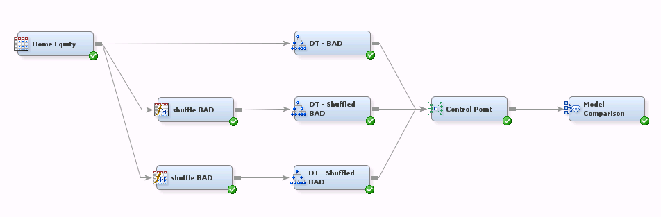
The values of BAD are shuffled for the simulation models using a bit of SAS code in the Transformation nodes. When the target is binary, shuffling the values is a simple matter: first determine the percentage of zeroes and ones in the training sample. Then “shuffle” the target values by randomly assigning 0's and 1’s in the same proportions. Prior to creating this flow I used the Graph Explore node to determine the category percentages: approximately 20% of the observations have the value BAD=1 and the remaining 80% have BAD=0.

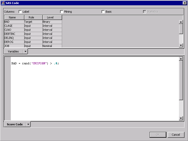
The same code snippet is used in both of the Transformation nodes. The code assigns zeroes and ones based on numbers randomly generated from a uniform (0,1) distribution. Notice that I didn't set a fixed seed for the random number generator. This means that the target values are shuffled independently for each simulation model.

If your target is nominal or interval level, you will need to shuffle the values. You can do this by sorting the observed target values and then merging them back to the original (unsorted) dataset. But regardless of your target measurement level, make sure you use simulated target values that have the same distribution as the observed target values.

Here's the tree diagram for the model predicting observed target values:

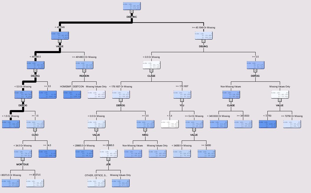
According to the Variable Importance table (not shown here), the most important predictors of Bad are debt-to-income ratio, delinquency and loan value.

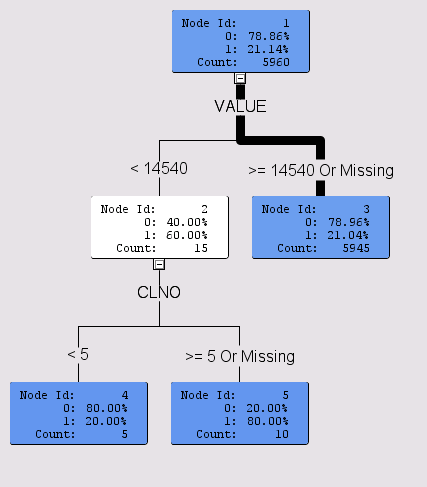
The trees produced by the two simulations are much simpler, but they did indeed identify relationships between the inputs and the shuffled targets.  For example, the first simulation identified VALUE and CLNO as differentiators of the shuffled target:

In the second simulation, LOAN and MORTDUE were found to differentiate the shuffled target:

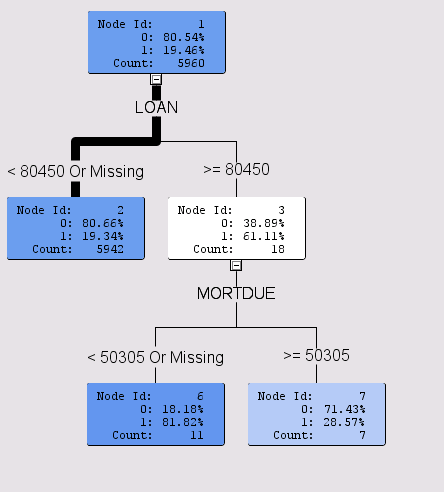
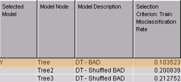
Remember, these are purely random relationships picked up by the decision tree algorithm. But the candidate model using BAD performed much better than both simulation models:

This manual approach to target shuffling is a good start, but to complete our simulation we need to shuffle the target values many times--say, 100 or more. And of course we’d like to do this without having to extend our flow manually, i.e., adding 98 more branches.

Using Group Processing Nodes

This simple flow uses the Group Processing nodes to generate 100 simulations:

Here, I’ve embedded the Transformation and Decision Trees nodes within the Start- and End-Groups nodes because we want to iterate over the portion of the flow that reassigns values of the target variable and builds decision trees.

The default mode for Start Groups is to stratify the analysis. Since we want iterative processing instead, we need to change the node properties as follows:

Here Mode=Index. I also set the Index Count to 100. This will give us 100 iterations (models) using simulated data.

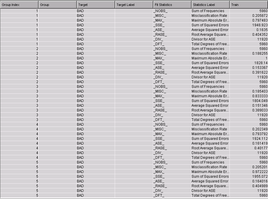
Run the flow and examine the results for the Decision Tree node. The Group Index column in the Fit Statistics table confirms that 100 models were generated (only the first models are shown here):

Since it’s much easier to see the distribution of assessment measures with a graph, I created this custom histogram based on the Fit Statistics table in Results view:

The histogram values represent the distribution of the misclassification rate for the 100 simulation models. The vertical reference line represents the model built using real target values.

The misclassification rate for the simulated target models ranges from .185 to .212, with a median of .20. The misclassification rate for our model is better (.1035) than that of any simulation, and is in fact a clear outlier. This gives us confidence that our candidate decision tree is not merely modeling spurious relationships.

In cases where the reference line and the histogram overlap, you would use the familiar “.05 rule”: you reject the null hypothesis that your model is only picking up on noise if it performs as well as or better than 95% of your simulations.

Here are the steps to reproduce the histogram:

1. Click on the Fit Statistics Table in Results view.

2. Click on the Plot icon in the toolbar or choose View > Plot from the menu.

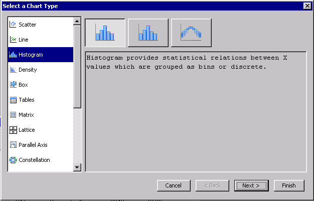
3. In the dialog that is shown, choose Histogram. Press Next.

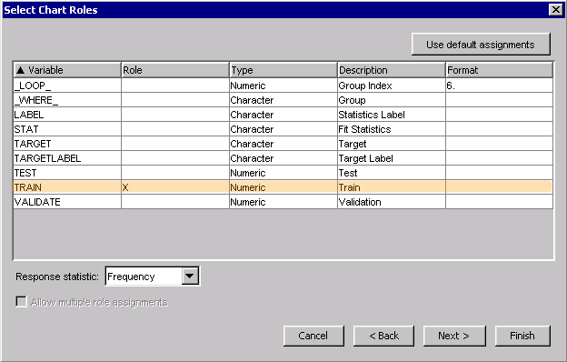
4. In the next screen, assign the Role of X to TRAIN. Press Next.

5. In the Where Clause screen, define the following condition.

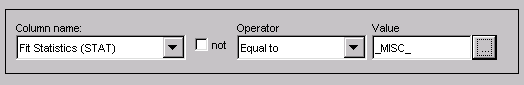
The Where clause limits the chart to rows containing misclassification rates. When you press Finish, the histogram is created.

You're almost done. Right click on the histogram and choose Graph Properties. Add the reference line for your candidate model and adjust the axis range in the Properties – Horizontal panel.

Summary

We’ve seen how to use the group processing facility to perform a simple Monte Carlo simulation.

To see for yourself, start by downloading the attached diagram, which reproduces the flows used in this example. Import the diagram into Enterprise Miner, by choosing File > Import Diagram From XML then choosing the diagram from the Open dialog box.

Index mode is a powerful, general-purpose group processing facility. Keep it in mind whenever you would otherwise find yourself rerunning the same flow repeatedly.

 

References

• 3 Ways to Test the Accuracy of Your Predictive Models (Victoria Garment)

http://plotting-success.softwareadvice.com/3-predictive-model-accuracy-tests-0114/

• The Power of the Group Processing Facility in SAS® Enterprise Miner™ (Sascha Schubert)

http://support.sas.com/resources/papers/proceedings10/123-2010.pdf

[quiphan]

Thanks for showing us the general-purpose group processing facility in the Monte Carlo Simulation. Some neat tricks are also provided eg writing SAS code in Transformation node, building Histogram with reference line of the simulation misclassifications. 

The XML file saves a lot of time to build the diagram. Cheers. Qui