- Home
- /
- SAS Communities Library
- /
- Tip: Getting the Most from your Random Forest
- RSS Feed
- Mark as New
- Mark as Read
- Bookmark
- Subscribe
- Printer Friendly Page
- Report Inappropriate Content
Tip: Getting the Most from your Random Forest
- Article History
- RSS Feed
- Mark as New
- Mark as Read
- Bookmark
- Subscribe
- Printer Friendly Page
- Report Inappropriate Content
It’s well known that high-definition television manufacturers fine-tune their products to look their best hanging on the display walls of big electronics stores. You need to adjust the settings on your new television to look its best in your living room to get the most from your investment. The same holds true for your modeling algorithms. Each application and data set presents different challenges and diverse relationships among the variables that really require adjustments to the various tuning parameters to build a more accurate predictive model, sometimes to a significant degree. In this tip we look at the most effective tuning parameters for random forests and offer suggestions for how to study the effects of tuning your random forest. A zip file containing the Enterprise Miner projects used in this study is provided for your experimenting pleasure.
Random Forest Overview
If you are familiar with decision trees and random forests, you may want to skip to the next section; otherwise, read on.
Decision trees are among the simplest (yet powerful) forms of models both conceptually and in their interpretation, with the entire data set of observations being recursively partitioned into subsets along different branches so that similar observations get grouped together at the terminal leaves of the decision tree. The partitioning is directed by determining the variable that most effectively increases the “purity” of the tree at each split point, meaning that observations with similar target value get separated from others. Ultimately the splitting terminates leaving you with leaf nodes with probabilities for predicted target values such that for any new observation the path of splitting rules through the tree can be followed to predict the target.
A random forest is an ensemble of a specific type of decision tree, an algorithm devised by Leo Breiman in 2001. So what are the distinguishing characteristics of the decision trees ensembled in a random forest?
- The decision trees in a random forest are overtrained by letting them grow to a large depth (default maximum depth of 50) and small leaf size (default smallest number of observations per node of 1). The theory behind this approach is that averaging the predicted probabilities of a large number of overtrained trees is more robust than using a single fine-tuned decision tree.
- The data used to train each tree is a random sample of the complete data set (with replacement)
- The input variables that are considered for splitting each node are a random subset of all variables (as opposed to all variables being candidates for defining the splitting rule), reducing bias toward the most influential factors and allowing secondary factors to play a role in the model

Scoring new observations on many trees enables you to obtain a consensus for a predicted target value (voting for classification, averaging for interval target prediction) with a more robust and generalizable model. A recent tip by Miguel Maldonado described various forms of ensemble models in SAS Enterprise Miner (Tip: Four Types of Ensemble Models and how to use them in SAS® Enterprise Miner™).

SAS Enterprise Miner provides a random forest algorithm through PROC HPFOREST, which can be included in your process flow using the HP Forest node. This procedure takes advantage of available computing resources by distributing the training of each tree to different nodes in a grid (if available) and exploiting all available computing power (i.e., multiple processors, multiple cores) on each machine through multi-threading, considerably reducing the time to train the entire forest.
Note: For a bit more in-depth (and fun!) walk-through of training random forest models, check out Cat Truxillo's YouTube video. It relies on the SAS Viya execution environment, but even if you don't have access to that you will probably gain some general insight on training random forest models.
Tuning Random Forests in SAS® Enterprise Miner™
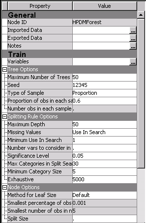
Tuning your random forest (or any algorithm) is a very important step in your modeling process in order to obtain the most accurate, useful, and generalizable model. The HP Forest node in Enterprise Miner provides the ability to tune your random forest through options categorized as general tree options, options governing the splitting rule at each node, and options for the tree nodes themselves as shown here.

SAS has set the defaults for these options to be most generally effective, but further adjustment can usually lead to better model accuracy. So that leads us to the main point of this tip: what are the most effective ways to tune a random forest?
Let’s first acknowledge that there is no way to know up front exactly how to set these options for any given data set. Instead, you need to arm yourself with knowledge of (a) what the options mean, and (b) how to efficiently study them for your data set. That is, consider the algorithm tuning an experimental procedure where you will need to train numerous models to gain insight on how to ultimately configure the algorithm options. Good descriptions for all of the tuning parameters can be found in the Enterprise Miner Reference Help (from the menu Help-->Contents-->HPDM Nodes-->HP Forest Node). Before we just dive in and start tweaking the knobs, let’s consider the main concepts behind a random forest.
Number of Trees
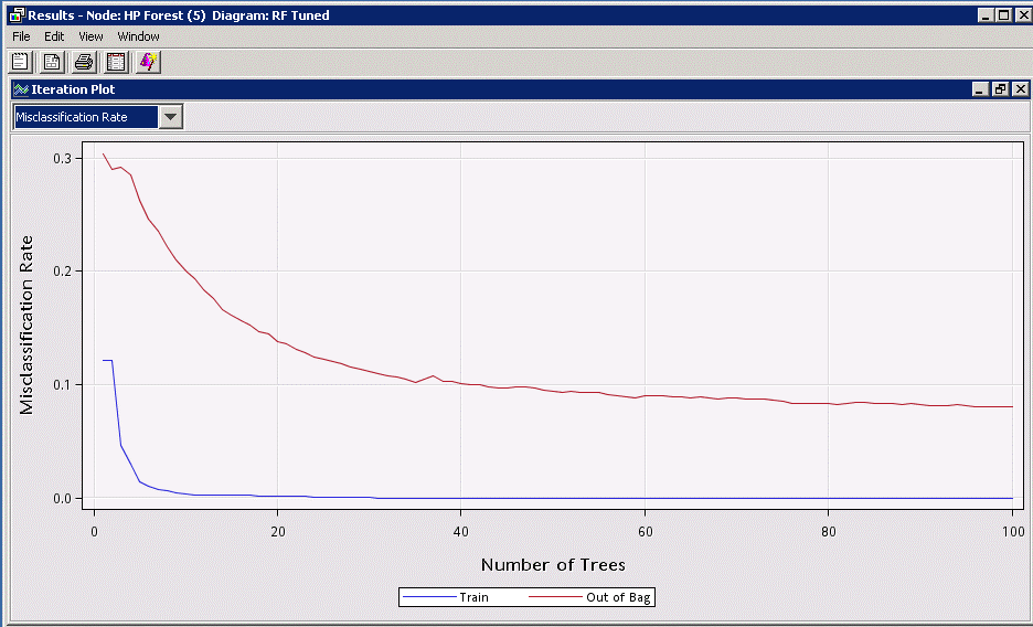
First of all, of course, the random forest is an ensemble of many decision trees, so it stands to reason that the number of trees will have a significant effect on the resulting model accuracy. Run the default HP Forest node with “Maximum Number of Trees” set to 100 and notice from the Iteration Plot that the number of trees has a significant positive effect on the model accuracy.
Note: In this study we did not include a separate validation set but instead assessed the model accuracy using the "Out of Bag" data, which is the subset of the data NOT used for training each individual tree (recall that different samples are used for training each tree). In this article we will focus on the "Out of Bag" assessment of the accuracy since it can be considered an unbiased and pessimistic representation of how your model will perform on new data. In general, a validation data set should be used.

This plot confirms what you expect – apart from the individual decision trees being overfit by design (significant difference between “Train” and “Out of Bag”), as you add more trees, your ensemble model becomes more accurate and generalizable. Note that there is an obvious point of diminishing returns (flattening of the curve) past around 40-50 trees, and by about 80 trees you are not gaining much accuracy for the extra cost (time and memory) of training. These rough thresholds will be different for each problem, and it is up to you to decide how finely you want to tweak the model; but just remember, the point is to generalize well, so fine tuning beyond say 0.1% misclassification is probably not worthwhile.
Number of Variables
Another key aspect of random forests is that the variables to consider for splitting each node are a random subset of all variables (as opposed to considering all variables). This reduces the bias toward the most influential variables and allows for a more generalizable model. So the question is, how many variables should be considered at each node? You can control this using the option “Number of variables to consider in split search”. Instead of manually changing this option over numerous training runs, you can use a programmatic approach to study the effect of tweaking this option.
Knowing that the HP Forest node runs PROC HPFOREST, you can write SAS code in the SAS Code node to study these algorithm options efficiently. This is one way you can code an efficient comparison of several HP Forest models:
- Use the “hpforestStudy” macro below to take a list of the number of variables to try (nVarsList) and the number of trees to train in the random forest.
- The macro loops over all numbers in the list, calling PROC HPFOREST multiple times (for different numbers of variables to consider), and gathering the fit statistics from the output.
Note: EM macros are used to reference the data set (%em_import_data), the list of interval inputs (%EM_INTERVAL_INPUT), and the target (%EM_TARGET).
3. The fit statistics of all your PROC HPFOREST models are saved into a data set that you can later use to visualize the performance of your models. To do this you can use the %em_register and the %em_report macros to create a plot that appears in the Results of your SAS Code node.
Note: Find simple examples of how to use the %em_register and %em_report macros in these tips:
Create Graphs in a SAS Code Node Using %em_report
Saving ODS Graphics in a SAS Code Node
%macro hpforestStudy (nVarsList=10,maxTrees=200);
%let nTries = %sysfunc(countw(&nVarsList.));
/* Loop over all specified number of variables to try */
%do i = 1 %to &nTries.;
%let thisTry = %sysfunc(scan(&nVarsList.,&i));
/* Run HP Forest for this number of variables */
proc hpforest data=&em_import_data maxtrees=&maxTrees. vars_to_try=&thisTry.;
input %EM_INTERVAL_INPUT /level=interval;
target %EM_TARGET / level=binary;
ods output fitstatistics=fitstats_vars&thisTry. ;
run;
/* Add the value of varsToTry for these fit stats */
data fitstats_vars&thisTry.;
length varsToTry $ 8;
set fitstats_vars&thisTry.;
varsToTry = "&thisTry.";
run;
/* Append to the single cumulative fit statistics table */
proc append base=fitStats data=fitstats_vars&thisTry.;
run;
%end;
%mend hpforestStudy;
%hpforestStudy(nVarsList=5 10 25 50 all,maxTrees=100);
/* Register the data set for use in the em_report reporting macro */
%em_register(type=Data,key=fitStats);
data &em_user_fitStats;
set fitStats;
run;
%em_report(viewType=data,key=fitStats,autodisplay=y);
%em_report(viewType=lineplot,key=fitStats,x=nTrees,y=miscOOB,group=varsToTry,description=Out of Bag Misclassification Rate,autodisplay=y);

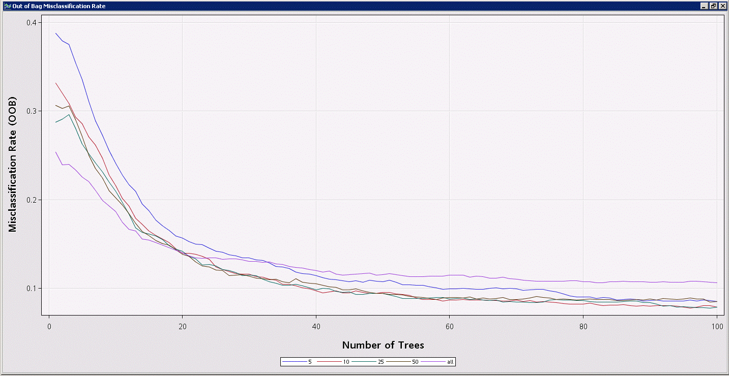
Note from the plot you created (plotting the variable “miscOOB” vs the variable “nTrees” grouped by the variable “varsToTry” in the fitstats data set) that the effect of changing the number of variables to use is not as directly intuitive as the effect of the number of trees. The plot suggests that for a low number of trees (which, of course, is not recommended for a random forest) you should consider all variables at each split – this makes sense, since with a small number of trees you need to make sure the most influential variables are considered. With a larger number of trees, the plot ultimately indicates that an intermediate number of variables (10-25) will provide the best model; anything too low carries the risk of missing out on the most influential variables too often, and anything too high allows the most influential variables to dominate too often, missing out on important secondary factors that allow the model to generalize better.
While it’s fair to say that an intermediate number of variables to try is likely the most effective, the actual value/range will be data dependent, as the number of features and their relative influence will vary. Note that Breiman suggests that the square root of the number of variables be used as a good default; the data set used for this tip contained 542 input features, which would lead you to start with 23 variables to consider – in line with our finding that 10-25 candidate variables gives us the best model.
This code is quite general and can be used in other Enterprise Miner projects to study the effect of this option on your random forest model.
Minimum Leaf Size
Let’s take a look at one more tuning parameter – the minimum leaf size, which specifies the smallest number of observations a node is allowed to have. If the splitting rule results in a child node with fewer observations than this number, the node is not split. This can be controlled either by setting an absolute value using the option “Smallest number of obs in node” or as a percentage of the total set of observations in the node being split using the option ”Smallest percentage of obs in node”. Here we will look at the absolute setting.
Use a similar approach to the study of the number of variables. You can reuse your SAS Code from your previous study as follows:
- Replace “nVarsList” with “leafsizeList”
- Change the proc hpforest call to
proc hpforest data=&em_import_data maxtrees=&maxTrees. leafsize=&thisTry.;
3. Replace “varsToTry” with “leafsize” in the data step following the proc hpforest call
4. Change “group=varsToTry” to “group=leafsize” in the %em_report call to create the graph
Your code will now look like this:
%macro hpforestStudy (leafsizeList=5,maxTrees=200);
%let nTries = %sysfunc(countw(&leafsizeList.));
/* Loop over all specified number of variables to try */
%do i = 1 %to &nTries.;
%let thisTry = %sysfunc(scan(&leafsizeList.,&i));
/* Run HP Forest for this number of variables */
proc hpforest data=&em_import_data maxtrees=&maxTrees. leafsize=&thisTry.;
input %EM_INTERVAL_INPUT /level=interval;
target %EM_TARGET / level=binary;
ods output fitstatistics=fitstats_vars&thisTry. ;
run;
/* Add the value of varsToTry for these fit stats */
data fitstats_vars&thisTry.;
length leafsize $ 8;
set fitstats_vars&thisTry.;
leafsize = "&thisTry.";
run;
/* Append to the single cumulative fit statistics table */
proc append base=fitStats data=fitstats_vars&thisTry.;
run;
%end;
%mend hpforestStudy;
%hpforestStudy(leafsizeList=1 3 5 10 15,maxTrees=100);
/* Register the data set for use in the em_report reporting macro */
%em_register(type=Data,key=fitStats);
data &em_user_fitStats;
set fitStats;
run;
%em_report(viewType=data,key=fitStats,autodisplay=y);
%em_report(viewType=lineplot,key=fitStats,x=nTrees,y=miscOOB,group=leafsize,description=Out of Bag Misclassification Rate,autodisplay=y);
Another option would be to combine the studies of these 2 tuning parameters into a single SAS Code node and use %em_report to create multiple graphs in the results.
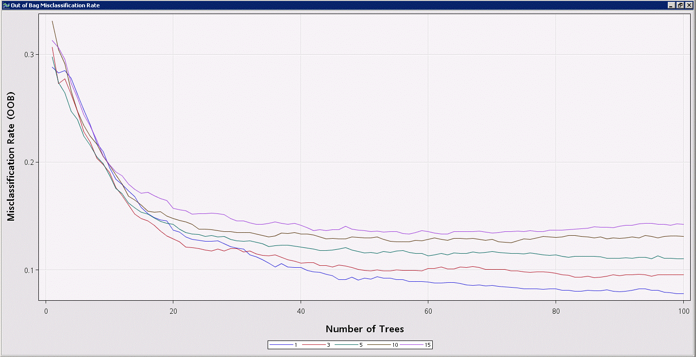
The plot shown below indicates that the effect of the minimum leaf size is quite clear…letting the trees split down to leaf nodes with a single observation results in the most accurate random forest models (in fact, the default for this value has just been changed from 5 to 1 in the upcoming release of Enterprise Miner 14.1). However, note that smaller leaf sizes means larger (deeper) trees, so accuracy again comes at the cost of computation time and memory.

Another random forest diagram example uses the publicly-available Mixed National Institute of Standards and Technology (MNIST) digits data set. Watch this video on random forests and support vector machines for an explanation of this example.
See code below used to access the MNIST digits data and the attached zip file for the associated EM diagrams.
filename traincsv url 'http://pjreddie.com/media/files/mnist_train.csv';
proc import
datafile=traincsv
out=train
dbms=csv
replace;
getnames=no;
run;

filename validcsv url 'http://pjreddie.com/media/files/mnist_test.csv';
proc import
datafile=validcsv
out=valid
dbms=csv
replace;
getnames=no;
run;
Conclusions
The point of this tip is not so much to tell you exactly how to tune your random forest model but instead to share a way in which you can efficiently and effectively study the effects of the tuning parameters using SAS code. You can see how this same methodology can be extended to the other modeling algorithms in Enterprise Miner quite easily (if you are unsure of what proc is run for a given node, place “options mprint;” in your project start code, run the node, and check the logs for that node). Keep in mind that you will need to use a Data Partition node and base your fit statistics comparison on the validation or test partition (which out-of-bag data was used for in our random forest assessment).
Now you can experiment for yourself. This post includes a zip file containing two Enterprise Miner diagrams (one for random forest and one for SVM) and the data used in these projects. Extract the contents of the zip file and then in Enterprise Miner use the Import Diagram from XML option in the File menu and select the appropriate xml file extracted from the zip file. You will also need to select the Data node and configure it to point to the appropriate file (banana.csv from the zip file for the SVM diagram) or data set (MNIST data set imported as described above for the random forest diagram).
Acknowledgements
Many thanks to Ray Wright for helping with the macros used in these studies.
References
Leveraging Ensemble Models in SAS® Enterprise Miner™
Tip: Four Types of Ensemble Models and how to use them in SAS® Enterprise Miner™
Breiman, L. 2001. “Random Forests”, Machine Learning 45: 123–140
- Mark as Read
- Mark as New
- Bookmark
- Permalink
- Report Inappropriate Content
Thank you very much for your brilliant work, Mr. Brett Wujek and Ms. Anna Brown. After tuning the hyperparameters in random forest I would like to tune them also in gradient boosting decision trees, but I could not find any information about how to achieve this goal by coding in SAS EM; what I could find is using SAS Viya Code Node in another software which my company doesn't own. My question is: is there any probability to tune GBDT by coding in SAS EM 14.3? If so, could you give a simple example or template about the syntax (I even cannot find any information about the syntax of gradient boosting process in SAS EM)? That will be really helpful to me. Thank you so much!
Don't miss out on SAS Innovate - Register now for the FREE Livestream!
Can't make it to Vegas? No problem! Watch our general sessions LIVE or on-demand starting April 17th. Hear from SAS execs, best-selling author Adam Grant, Hot Ones host Sean Evans, top tech journalist Kara Swisher, AI expert Cassie Kozyrkov, and the mind-blowing dance crew iLuminate! Plus, get access to over 20 breakout sessions.
Free course: Data Literacy Essentials
Data Literacy is for all, even absolute beginners. Jump on board with this free e-learning and boost your career prospects.

