Condition Monitoring and Anomaly Detection for High-Frequency Multivariate IoT Data

[#1]

Have you ever been asked to find the ‘smoking gun’ for a high-cost critical asset failure? What about identifying predictive asset degradation patterns? Were you using high-frequency multivariate data, making the exercise feel more like you were looking for a ‘smoking needle’ in a haystack? I have. It wasn’t easy.

Fortunately SAS’ Advanced Analytics R&D group released several new machine learning algorithms in 17W12 designed for condition monitoring and anomaly detection of high-frequency multivariate data. SAS’ new Support Vector Data Description (SVDD) procedure will speed up your ‘smoking gun’ investigation efforts by generating one output model instead of dozens, if not hundreds, typically created. As of May 23rd, you can export the resulting SVDD score code directly into SAS Event Stream Processing (ESP) to easily detect and alert these system anomalies in near real-time.


Traditional Asset Degradation Investigation Approaches

So you can appreciate how slick the new SVDD procedure is, let’s consider typical approaches for condition monitoring and anomaly detection for high-frequency multivariate data.

The data showcased in this blog is NASA’s 2008 Prognostics and Health Management Challenge Data Set (PHM08) simulating turbofan engine degradation. The data contains 26 variables including: engine ID, cycle number, three operational settings, and 21 sensor measurements. The data contains 218 different engines with end of useful life ranging between 128 and 357 engine cycles. The training data contains the first 25% of engine cycle sensor measurements for 30 randomly sampled engines. The validation data contains all data for the remaining 188 engines. We assume that this data represents normal operating conditions.

Typically analysts start with visual and descriptive modeling approaches to perform condition monitoring and anomaly detection. I like to use JMP for initial explorations. The following video showcases common JMP tools used to explore and identify asset degradation. 

Another approach is leveraging SAS/QC MVP procedures. If your multivariate data is correlated, using multivariate statistical process monitoring methods is appropriate. The following video showcases condition monitoring and anomaly detection using MVPMODEL, MVPMONITOR, and MVPDIAGNOSE procedures which generate T2 and SPE charts to summarize asset performance and variation. For more information about MPV procedures, please refer to the Global Forum 2012 paper (318-2012) by J. Blair Christian and Bucky Ransdell. Please note the MVP approach assumes your data follows multivariate normal distribution.


 


   Identify Asset Degradation and Unstable Operation using Support Vector Data Description (SVDD)


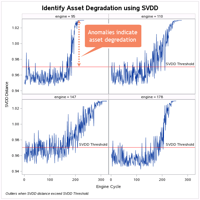
Now let’s see how to use SAS’ new Support Vector Data Description (SVDD) procedure to find the ‘smoking gun’. In my opinion, SVDD can help you find the signal in the noise faster and more simply. Not only does it work really well on multivariate data, it does not require your data be normally distributed. Plus it greatly reduces the number of output charts needed for an investigation, potentially down to one. Here is an example SVDD output chart that quickly and effectively demonstrates how a turbo fan degrades over its life span.





What is SVDD?

Before we begin, are you wondering what is SVDD? How’s it different than Support Vector Machine (SVM)? Why would we use SVDD for anomaly detection?

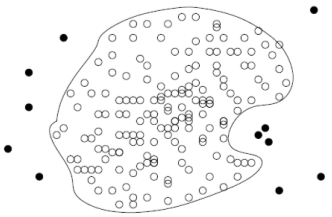SVDD is a one-class classification technique useful in domains where the majority of the data belongs to one class and the other class is scarce or missing at the time of model building. Fraud detection, equipment health monitoring, and process control are some examples of application areas where the majority of the data belongs to one class. This picture illustrates a typical one-class model scenario where the unfilled markers are "normal" and the filled markers are "anomalies". SVDD will identify a decision boundary that can distinguish "normal" data from anomalies.

SVM is inherently a two-class classifier.

The main difference between SVDD and SVM is that SVDD constructs a closed hypersphere around the class of interest (i.e. the target class). If an observation is excluded by the area of the hypersphere, it will not be assigned as "target" class, rather it will be assigned to the so called "outlier" class. In contrast, SVM finds the best hyperplane between two classes where sufficient data representing both classifiers are required to obtain a good model.

Since outliers and anomalies are hopefully infrequent, you can use SVDD to model one-class system data and subsequently use the model to perform anomaly detection.

How to use SVDD?

SVDD is currently available in SAS Visual Data Mining and Machine Learning 8.1 on SAS Viya 3.2 as a CAS action set and SVDD procedure, including a prebuilt drag-and-drop SVDD task. All three approaches are really easy to use. Let me walk through some simple code to perform condition monitoring and anomaly detection on NASA's PHM08 turbofan engine degradation data.

First, access a SAS Viya 3.2 environment. Import your data. Then update the following macros to point to your data.
%let path=/home/sasdemo/casuser/; /* specify the location of your input file */
%let input_file=engine_data.sas7bdat; /* specify the name of input file and type */
%let partition_flg=flag; /* specify the training/validation partition variable */
%let training_flg="Training"; /* specify training data partition identifier */
%let validation_flg="Validation"; /* specify validation data partition identifier */
%let xaxis_var=cycle; /* specify x-axis (time, cycle, etc.) variable */

Start a CAS session and load your data into CAS.

cas;
caslib _all_ assign;
proc casutil;
    load file="&path&input_file" casout="raw_data";
run;

Define your training and validation data.

data casuser.data_p;
    set casuser.raw_data;
    format partition $10.;
    partition = &partition_flg;
    drop &partition_flg;
    where &partition_flg eq &training_flg or &partition_flg eq &validation_flg;
run;

Create a list of variables in your data file.

proc contents data=casuser.raw_data noprint out=metaclass;
run;
proc sql;
    select name
    into :vars separated by " "
    from work.metaclass
    where name not in ("&xaxis_var", "&partition_flg", "engine");
quit;

Next, you need to determine the value for the bandwidth parameter (also known as the radial basis function or Gaussian kernel function). It is the most critical hyperparameter value to tune in SVDD. The kernel function it what provides SVDD the ability to have a flexible data description which follows the geometry of your data. The value must be a positive nonzero real number. In future releases, tuning the SVDD bandwidth parameter will be fully automated. At this time, it's a manual operation. Here is some code to select the value of your Gaussian bandwidth parameter value using the peak criteria.

/* Create temporary summary table to store SVDD bandwidth parameter options */
proc sql noprint;
    create table work.summary (s num, sv num, radius num, time num);
quit;

/* Determine the value of the Gaussian bandwidth parameter using Peak Criteria */ 
  %let sby=0.2;
%macro summary;
%do i=10 %to 75;
    %let s=%sysevalf (&i*&sby);
    ods listing close;
    ods output trainingresults=tr_&i;
    proc svdd data=casuser.data_p nthreads=4;
       input &vars/level=interval;
       where partition = &training_flg;
       id _all_;
       solver actset;
       kernel rbf / bw=&s;
    run;
    %local nsv;
    %local radius;

   proc sql noprint;
       select value into :nsv
       from tr_&i
       where Description = "Number of Support Vectors";

       select value into :radius
       from tr_&i
       where Description = "Threshold R^2 Value";

       select value into :time
       from tr_&i
       where Description = "Run Time (Seconds)";

       insert into work.summary
       values(&s, &nsv, &radius, &time);

   quit;
    %end;
%mend summary;
%summary;

/* Identify optimal bandwidth parameter value */
proc sort data=work.summary;
    by s;
run;
data work.summarize;
    set work.summary;
    label d_r="First Derivative" d2_r="Second Derivative" radius="SVDD Radius";
    if _n_ > 1 then d_r = (radius - lag(radius)) / (&sby);
    if _n_ > 2 then d2_r = (radius - 2*lag(radius) + lag2(radius)) / (&sby*&sby);
run;

data work.summarize_up;
    set work.summarize;
    if _n_ > 1 then do; 
       if d2_r > 0 and lag(d2_r) < 0 then flag=1;
else if d2_r < 0 and lag(d2_r) > 0 then flag=1;
       else flag = 0;
    end;
run;

/* Save optimal bandwidth parameter value as &optimal */
proc sql;
    select min(s) into :optimal
    from work.summarize_up
    where flag = 1;
quit;

/* Save threshold radius associated with optimal bandwidth parameter value as &threshold */
proc sql;
    select radius into :threshold
    from work.summary
    where s = &optimal;
quit;

/* Plot the values of the first and second derivative of radius = f[s] */ 
proc sgplot data=work.summarize;
    title H=14pt "Optimal Bandwidth Parameter Value";
    footnote H=8pt j=l italic "Optimal Bandwidth Parameter when radius function's second derivative crosses zero.";
    series x=s y=d2_r / lineattrs=(color=blue thickness=2) y2axis;
    series x=s y=radius / lineattrs=(color=purple pattern=dash);
    series x=s y=d_r / lineattrs=(color=orange pattern=dash) y2axis;
    refline 0 /axis=y2 label="BW Threshold" lineattrs=(color=black) labelloc=inside;
    refline &optimal / axis=x lineattrs=(color=black) labelloc=inside;
    inset "Optimal BW value = &optimal" / border position=bottomleft;
    y2axis label="SVDD Radius First & Second Derivate Values";
    yaxis label="SVDD Radius Values";
    xaxis label="Bandwidth Parameter Values";
run;

The following plot shows the Gaussian bandwidth parameter value (s) on x-axis versus SVDD radius values tested on the y1-axis, and first & second derivate SVDD radius values on the y2-axis. We select the value of s where the second derivative SVDD radius function value equals zero.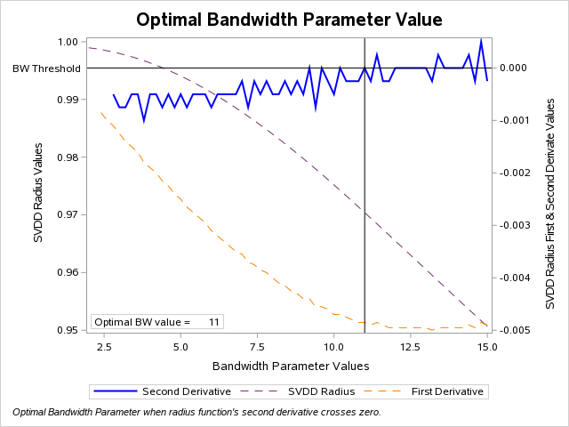

   

Now you need to update your SVDD model using the optimal bandwidth parameter value.
proc svdd data=casuser.data_std nthreads=4;
  input &vars / level=interval;
  where partition = &training_flg;
  id _all_;
  solver actset;
  kernel rbf / bw=&optimal;
  savestate rstore=casuser.state_s;
run;

Now you can score and plot your updated SVDD model using validation data.

proc astore;
    score data=casuser.data_p out=casuser.all_out rstore=casuser.state_s;
run;

proc sgplot data=casuser.all_out;
    title H=14pt "Anomaly Detection using SVDD";
    footnote H=8pt j=l italic "Anomalies when SVDD distance exceed SVDD Radius Threshold.";
    series x=&xaxis_var y=_SVDDdistance_;
    refline &threshold / label="SVDD Radius Threshold" lineattrs=(color=red) labelpos=max;
    where engine = 5;
run;

Here is an example of a single SVDD output chart needed to investigate asset degradation. SVDD Distance (_SVDDdistance_) is one of two SVDD scoring output variables. The other is _SVDDscore_. Plotting SVDD Distance against engine cycle, or another time equivalent variable, is an easy way to perform conditioning monitoring to track asset degradation.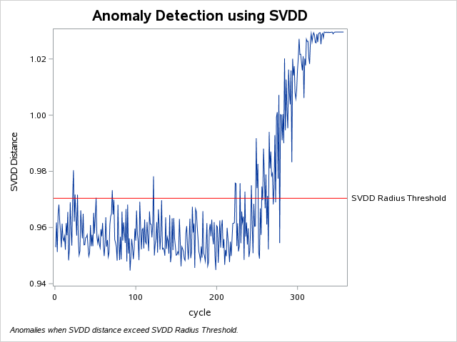



NOTE: In this example, we found better results were achieved by not standardizing the multivariate data prior to running SVDD. However, in other applications, you may want to try standardizing multi-scaled data to achieve better results. Please refer to my blog <INTERNAL LINK> "To standardize data or not to standardize data – that is the question" for more information about standardizing data, including sample CAS action code.

As illustrated above, SVDD quickly and easily generated a single output chart that effectively alerted turbofan engine asset degradation. As of May 23rd, you can export the resulting SVDD score code directly into SAS ESP to alert system anomalies and identify asset degradation in near real-time.

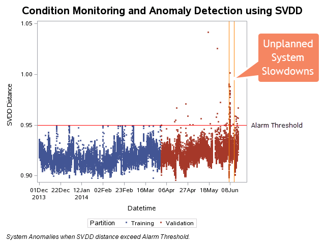
We also tested the SVDD approach on high-frequency multivariate data from a chemical manufacturing process. In order to train your SVDD model, you must know how to define "normal" operation. We recommend working with the customer's subject matter expert to get this information. Since we could not define an exact period of time with stable "normal" operation for the chemical plant data, we increased the SVDD outlier fraction parameter to 0.01. SVDD's outlier fraction parameter is inversely proportional to the penalty function controlling the trade-off between hypersphere volume and modeling accuracy. For our test, this worked extremely well. However, in other applications, please consult with the customer's subject matter expert for their recommendations. Here is the resulting SVDD output chart which clearly detected unstable system operation prior to the chemical manufacturing process' unplanned system disturbances on June 7th and June 12th.



To summarize

Support Vector Data Description (SVDD) is a new machine learning algorithm well suited for performing condition monitoring and anomaly detection for high-frequency multivariate data. The algorithm is now available in SAS Visual Analytics Data Mining and Machine Learning 8.1 on SAS Viya 3.2. It is extremely easy to use. It generates one output that quickly and easily detect system anomalies and can be easily integrated into SAS ESP.

Looking for more information about SVDD? Please take a look at our NEW VLE workshop: Visual Statistics 8.1 | Visual Data Mining and Machine Learning 8.1 on SAS Viya 3.2: Essentials which includes information about SVDD, including a hands-on lab.

Acknowledgements:

I would like to say a special thank you to Ryan Gillespie, Dev Kakde, Arin Chaudhuri, Gul Ege, Byron Biggs and Anya McGuirk for their technical assistance developing the code included in this blog and confirming optimal SVDD configurations.