- Home
- /
- Programming
- /
- Programming
- /
- Re: overlay two different plots
- RSS Feed
- Mark Topic as New
- Mark Topic as Read
- Float this Topic for Current User
- Bookmark
- Subscribe
- Mute
- Printer Friendly Page

- Mark as New
- Bookmark
- Subscribe
- Mute
- RSS Feed
- Permalink
- Report Inappropriate Content
Hi,
How would you overlay these two plots ?
One is made with sgrender and the other with gmap
proc template;
  define statgraph krigemap;
  begingraph;
  title "Ordinary kriging of &selectgerm";
  layout overlay /
  xaxisopts=(display=none)
  yaxisopts=(display=none) ;
  scatterplot x = x y = y /
  /*markerattrs=(symbol=squarefilled)*/
  markercolorgradient = z
  name = "heatmap" ;
  continuouslegend "heatmap" /
  orient = vertical
  location = outside;
  endlayout;
  endgraph;
  end;
  run;
proc sgrender data=epistat.tmp_surface template=krigemap;run;
PROC GMAP GOUT=MAPCHART DATA=WORK.MAPCHARTRESPONSEPREP MAP=WORK.MAPCHARTMAPPREP ALL;
  ID _ID_;
  CHORO Calculation /
  WOUTLINE=1
  NOLEGEND ;
RUN;
QUIT;

- Mark as New
- Bookmark
- Subscribe
- Mute
- RSS Feed
- Permalink
- Report Inappropriate Content
Hi.
Is is possible for you to create the heatmap with a gplot, instead of GTL?
Here is a quick reference:
http://robslink.com/SAS/democd22/heatmap.sas
You could then use PROC GREPLAY to combine the two plots;
Anca.
- Mark as New
- Bookmark
- Subscribe
- Mute
- RSS Feed
- Permalink
- Report Inappropriate Content
If it's possible I was searching for making a map with GTL.
I'll try this tomorrow, thanks

- Mark as New
- Bookmark
- Subscribe
- Mute
- RSS Feed
- Permalink
- Report Inappropriate Content
Hi Mathias,
Did you find the way to overlay these two plots ?
I will be interessted by your solution...
Cheers,
JB
- Mark as New
- Bookmark
- Subscribe
- Mute
- RSS Feed
- Permalink
- Report Inappropriate Content
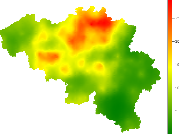
Hi,
I found a complicated workaround to obtain this with ods graphics only:

It's awfull because the borders are not continuous and the black background is not removable
(never found the way to do it at least. No one else is working on this spécific subject it seems)
I have come to the conclusion that this is the best I'll get with SAS.
Here is the idea behind it:
-merge the two data sets together wit no common variable -> creates a two-block dataset with a lot of empty cells
-proc template / proc sgrender, with a contourplotparm on the real map and a scatterplot on the boundaries
I can send you the code if you want.
- Mark as New
- Bookmark
- Subscribe
- Mute
- RSS Feed
- Permalink
- Report Inappropriate Content
Hi Mathias,
I am interested by your codes and by the resulting output.
One solution should have been to use the SGRend and an annotate dataset (for the country border outline)...
But it seems than proc sgrender do not support annotate...
i will have the same problem in the next month maybe i will find an elegant solution to our problem ?
I wondered if your are belgian and you are coming from the wallonian part, it could more relevant to speak in French ?
Cheers,
jb
JB
- Mark as New
- Bookmark
- Subscribe
- Mute
- RSS Feed
- Permalink
- Report Inappropriate Content
No, don't speak French.
I want to follow this thread.
![]()
- Mark as New
- Bookmark
- Subscribe
- Mute
- RSS Feed
- Permalink
- Report Inappropriate Content
Yes, walloon region and french speaking. But i'll continue in english as asked.
Sorry for the map, it didn't appear in my last post.
Here it is :
(the borders are not continuous and the black background is not removable)
Contact me by mail and I'll send you code mathias.leroy[at]wiv-isp[dot]be, i'am not sure I can open source my work like that.
proc template;
define statgraph krigeplot_prov;
begingraph;
title;footnote;
title &title;
title2 &title2;
footnote &footnote;
footnote2 &footnote2;
rangeattrmap (...) ;
rangeattrvar (...) ;
layout overlay (...) ;
contourplotparm (...) ;
continuouslegend (...) ;
scatterplot (...) ;
endlayout;
endgraph;
end;
run;
PROC SQL;
CREATE TABLE _2E AS
...
OUTER UNION CORR
....
;quit;
proc sgrender data=_2E template=krigeplot_prov
;run;quit;
- Mark as New
- Bookmark
- Subscribe
- Mute
- RSS Feed
- Permalink
- Report Inappropriate Content
And I'm of course interested if you find an better elegant solution.
I'am almost certain you'll not find it in ods graphics, maybe with the annotate function of proc gmap in SAS/GRAPHS like you said in the other discussion.
Or maybe with upcoming proc sgmap and proc template enhancements.
- Mark as New
- Bookmark
- Subscribe
- Mute
- RSS Feed
- Permalink
- Report Inappropriate Content
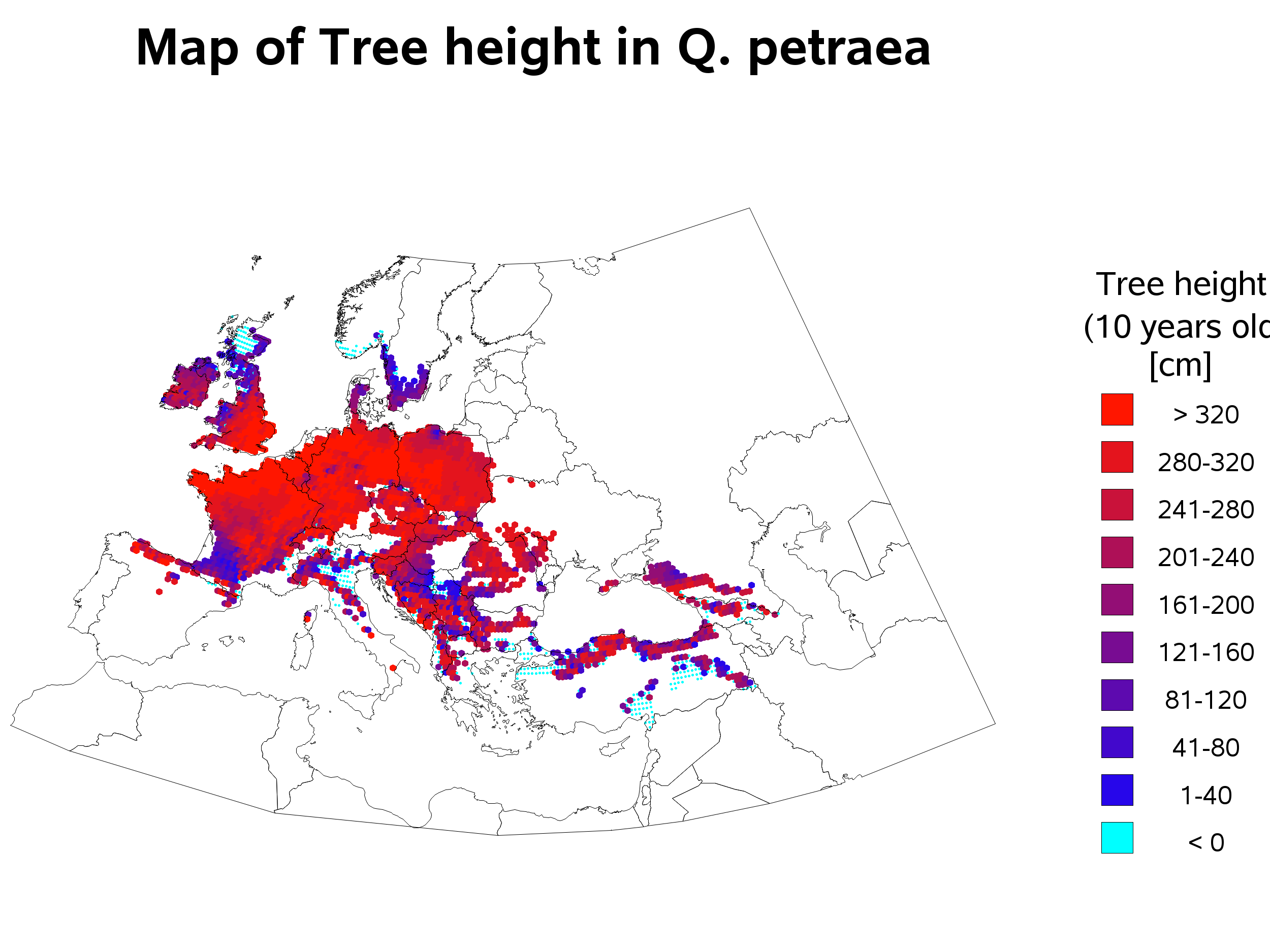
Dear Mathias,
Here attached the code to plot a continuous variable over a map. This solution is non-optimal... but it is only solution that i found in the Robert Allison's book. The Allison web site is full of code sample... it is always good to look for a solution there : Robert Allison's SAS/Graph Examples!
The result (code is below)
*1- import data "without transfert" models ;
proc IMPORT OUT= WORK.a DATAFILE="&path_in.&root.&trait..txt" DBMS=tab REPLACE;
guessingrows = 5000 ; RUN;
%let year = 2100 ;
data rawa;
set a(where =(year =&year.)) ;
*"-1" is a USA convention, which is quite annoying ;
x=-1*(lon/(180/constant('pi')));
y=lat/(180/constant('pi'));
anno_flag =1 ;
keep &trait. x y anno_flag ;
run;
proc means data = rawa ;
var &trait. ;
run ; quit ;
*2- import data from world maps ;
data mymap;
set maps.world;
label x='x';
label y='y';
x=long;
y=lat;
run ;
*3- merge data before projection ;
*column in each data set &trait x y segment flag... some like that !!! ;
data combined ;
retain cont id segment x y &trait. ;
set mymap rawa ;
run ;
*4- projected all the data in on shot ;
proc gproject data = combined out = combined latmin=30 latmax=65 longmin=-60 longmax=10 project=albers ;
*By default it is in radians as my dataset BUT using lambert projection, it should be degrees ;
id id;
run;
data mymap rawa ;
set combined ;
if anno_flag then output rawa ;
else output mymap ;
run ;
*Re-construct a "segment" variable to be unique ;
data mymap ;
set mymap ;
segment = (id*10000 + segment) ;
keep x y segment anno_flag;
*if _n_ > 200 then delete ;
run ;
*Rename each segment variable to continous from 1 to the end ;
proc iml ;
use mymap ;
read all var _all_ into b ;
row_b = nrow(b) ;
new = j(row_b,1,-999) ;
meno = b[1,3] ;
com = 1 ;
do i = 1 to row_b ;
if b[i,3] = meno then do ;
new[i,1] = com ;
end ;
else do ;
com = com + 1 ;
new[i,1] = com ;
meno = b[i,3] ;
end ;
end ;
colname = {"x" "y" "segment" "flag"} ;
tot = b[,1:2]||new||b[,4] ;
create tot2 from tot[colname = colname] ;
append from tot ;
quit ;
data annoa ;
set rawa(keep = x y &trait. anno_flag ) ;
length function style color $8 text $30;
xsys='2'; ysys='2'; hsys='3'; when='b';
function='pie'; style='psolid'; position='5'; rotate=360; size=.3;
if &trait. < 0 then do ;
color="CX00FFFF"; /* negative growth */
size = .1 ;
end ;
else if &trait. <= 10 then color="CX2706EA";
else if &trait. <= 20 then color="CX5D0AAF";
else if &trait. <= 30 then color="cx930E75";
else if &trait. <= 40 then color="cxC9123A";
else if &trait. > 40 then color="cxFF1600";
run;
*annotate a legende ;
data legend_text;
input mytext $ 1-12 color $ 14-21 x y;
datalines;
< 0 CX00FFFF 88 10
0-10 CX2706EA 88 15
10-20 CX5D0AAF 88 20
20-30 cx930E75 88 25
30-40 cxC9123A 88 30
> 40 cxFF1600 88 35
;
run;
proc sort data= legend_text ;
by x descending y ; run ;
data legend_text; set legend_text;
length function color $8 style $25 text $20;
xsys='3'; ysys='3'; hsys='3'; when='a';
position='B';
function='label'; size=4; text='U';
style='marker'; output;
color="black"; style='markere'; output;
function='label'; color="black";
text=mytext;
x=x+7; y=y+.5;
style=''; size=2.75; output;
run;
data legend_title;
length function color $8 style $25 text $20;
xsys='3'; ysys='3'; hsys='3'; when='a';
function='label'; size=4; text='U';
position='B';
style=''; size=3.5; x=88+7-2;
text='growth rate '; y=64.5; output;
text='[cm/year]'; y=60.5; output;
run;
/* This white legend-box covers some of the colored elevation data (behind the legend) */
data legend_box;
length function style color $8;
xsys='3'; ysys='3'; hsys='3'; when='b';
color='white';
style='msolid';
function='poly';
x=85; y=0; output;
function='polycont';
x=100; y=0; output;
x=100; y=88; output;
x=85; y=88; output;
run;
data anno_legend ;
set legend_box legend_text legend_title ;
run ;
%let name=nt_&year._&trait. ;
goptions reset=all ;
goptions device=png ;
goptions /*xpixels=800 ypixels=515*/ ;
goptions noborder;
ODS LISTING CLOSE;
ODS HTML path=odsout body="&name..htm" style=htmlblue image_dpi = 300 ;
goptions gunit=pct ftitle="albany amt/bold" htitle=5.5 ftext="albany amt" htext=3.5;
title1 move=(-8,+0) ls=1.3 'Map of growth rate in Q. petraea';
title2 a=-90 h=24 ' ';
pattern v=empty c=black;
proc gmap data=tot2 map=tot2 anno=annoa;
id segment;
choro segment / levels=1 nolegend
anno=anno_legend /*html=htmlvar*/
des='' name="&name";
run;
quit;
ODS HTML CLOSE;
ODS LISTING;

Don't miss out on SAS Innovate - Register now for the FREE Livestream!
Can't make it to Vegas? No problem! Watch our general sessions LIVE or on-demand starting April 17th. Hear from SAS execs, best-selling author Adam Grant, Hot Ones host Sean Evans, top tech journalist Kara Swisher, AI expert Cassie Kozyrkov, and the mind-blowing dance crew iLuminate! Plus, get access to over 20 breakout sessions.
Learn how use the CAT functions in SAS to join values from multiple variables into a single value.

Find more tutorials on the SAS Users YouTube channel.
 Click image to register for webinar
Classroom Training Available!
Select SAS Training centers are offering in-person courses. View upcoming courses for:
-
9 replies
-
12-13-2012 09:17 AM
-
2620 views
-
3 likes
-
3 in conversation
-
